- Vistas
- Introducción
- Crear una Vista
- Propiedades de una vista en gvSIG
- Añadir una capa a gvSIG
- Introducción
- Añadir una capa desde fichero en disco
- Añadir capa a través del protocolo WFS
- Introducción
- Conexión al servidor
- Acceso al servicio
- Selección de "Capas"
- Selección de "Atributos"
- Pestaña "Opciones"
- Crear un filtro
- Añadir una capa WFS a la vista
- Modificación de las propiedades de la capa
- Añadir capa a través del protocolo WMS
- Introducción
- Conexión al servicio
- Acceso al servicio
- Selección de "Capas"
- Selección de "Estilos" sobre las capas del servidor WMS
- Selección de valores para las "Dimensiones" de una capa WMS
- Selección de formato, sistema de coordenadas y/o transparencia
- Añadir una capa WMS a la vista
- Modificación de las propiedades de una capa
- Añadir una capa a través del protocolo WCS
- Introducción
- Acceso al servicio
- Selección de "Coberturas"
- Selección de "Formato"
- Añadir la capa WCS a la vista
- Modificación de las propiedades de una capa
- Añadir una capa a traves del protocolo ArcIMS
- Introducción a ArcIMS
- Conexión a servicios de imágenes
- Carga de una capa a través de ArcIMS
- Cargar una capa usando el protocolo arcims
- Conexión al servidor
- Acceso al servicio
- Selección de capas
- Añadir la capa a la vista
- Consideraciones a tener en cuenta respecto a los sistemas de referencia
- Modificación de las propiedades de la capa
- Información sobre los límites de escala
- Consulta de información de atributos
- Conexión a servicios de geometrías
- Carga de una capa de geometrías
- Simbología en ArcIMS
- Símbolos
- Leyendas
- Trabajo con la capa
- Añadir ortofotos a traves del protocolo ECWP
- Crear una nueva capa
- Añadir capa de Eventos
- Introducción
- Añadir capa de eventos desde una tabla nueva
- Añadir capa de eventos desde una tabla asociada a una capa de la vista
- Propiedades de la capa
- Introducción
- Capa vectorial
- Cambiar el color de una capa añadida
- Cambiar el nombre a una capa añadida
- Propiedades
- Introducción
- Usar índice espacial
- Rango de escalas
- Resumen de las propiedades de las capa y su ruta de localización
- Crear un hiperenlace en una capa
- Editor de leyendas
- Capa raster
- La tabla de contenidos (T.O.C) de gvSIG
- Navegar/Explorar la vista
- Configurar localizador
- Herramientas de consulta
- Selección de elementos
- Introducción
- Selección por punto
- Selección por rectángulo
- Selección por polígono
- Selección por capa
- Selección por atributos
- Invertir selección
- Borrar selección
- Localizador por atributo
- Centrar la vista sobre un punto
- Catálogo. Búsqueda de geodatos
- Nomenclátor
- Eliminar capas
- Exportar capa
- Introducción
- Exportar a shape
- Exportar a dxf
- Exportar a postgis y Oracle
- Exportar a gml
- Exportar a raster
- Exportar a imagen y WMC
- Capa de anotaciones
- Introducción
- Crear una capa de anotaciones
- Edición de una capa de anotaciones
- Propiedades de la capa de anotaciones
- Añadir la capa de anotaciones a la vista
- Ejemplo de creación de capa de anotaciones
- Tratamiento de imágenes ráster
Vistas
Introducción
Views are the gvSIG documents used as the working area of cartographic information.
A view can contain different layers of geographic information (hydrography, transport infrastructures, administrative regions, contour lines, etc.).
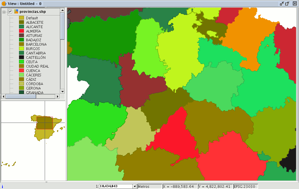
When one of the views that make up a project is opened, a new window appears divided into the following parts:
Table of contents (ToC): The ToC is located on the left-hand side of the window. The Table of Contents lists all the layers it contains and the symbols used to represent the elements which make up the layer.
Display window: The display window is located on the right-hand side of the screen. The project’s cartographic data are shown in this display window.
Locator: The locator is situated in the bottom left-hand corner. The locator allows the current frame to be situated in the work area as a whole.
When a view is opened, the main window increases the number of menus and buttons, thus adding the tools required to work with the elements which make up the view.
The size of the ToC can be enlarged to show a full description of all the themes by simply dragging its edge to the right or downwards.
Crear una Vista
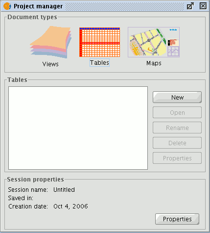
To create a “View” in gvSIG go to the “Project Manager” window (“Show” menu / “Project window").
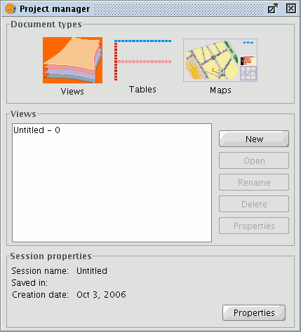
Project manager
- 1. In the “Project manager” window, select “Views” in the document type.
- 2. Then click on the “New” button.
- 3. A document in “Views” is created (immediately) which by default is called “Untitled - 0”.
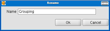
- 4. The name of the “View” can be changed by selecting the document from the list and clicking on the “Rename” button. A window appears in which the name of the “View” can be changed.
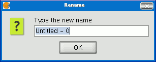
Rename View
5. To access the “View properties” window, click on the “Properties” button.
- 5.1. It is important to select the cartography units and the distance units for the “View”. Their default values are expressed in metres.
- 5.2. The “View” background colour can be configured. It is white by default.
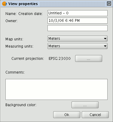
- 5.3 From gvSIG version 0.3 onwards, the “Views” support different projections and reference systems. You must select the reference system the cartographic information is to be displayed with.

Propiedades de una vista en gvSIG
To access the properties window of a view, go to the “View” menu and select “Properties”.
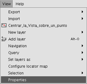
The properties you wish your view to have can be configured via the following window.
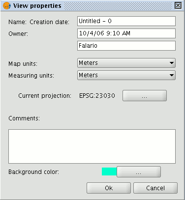
If you click on the “Current projection” button, a new window will appear in which the view’s datum, projection and time zone can be selected.
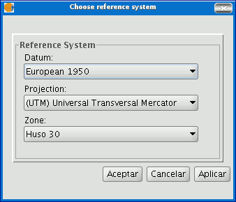
If you click on the pull-down menus, the different options available for each element in the reference system are shown. If you make any changes, click on “Apply” and then “Ok”.
When you have configured the view’s properties, click on “Ok”.
Añadir una capa a gvSIG
Introducción
Firstly, open a “View” document in gvSIG.
You can access this option by going to the "View" menu and then to "Add layer" or by using the “Control + O” key combination
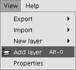
or by clicking on the "Add layer" button in the tool bar.

A window appears in which you can select and configure the layer's data source by its type:
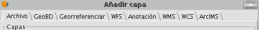
Añadir una capa desde fichero en disco
Añadir capa desde fichero en disco
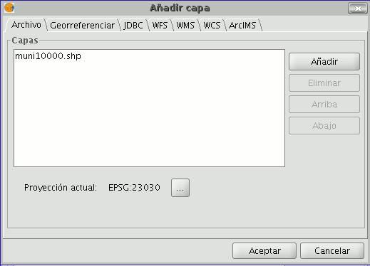
Click on the "Add" button
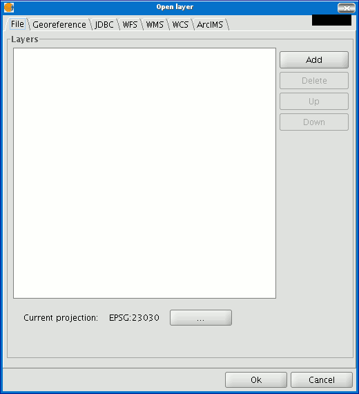
Seleccionar tipo de capa (Selección de driver)
The "Add” dialogue window allows you to move around the file system to select the layer to be loaded. Remember that only the files of the type selected will be shown. To indicate the type of file to be loaded, select a file from the “Files of type” pull down menu.
If several layers are loaded at the same time, the order in which the themes will be added to the view can be specified with the "Up" and "Down" buttons in the “Add layer" dialogue.
Añadir capa a través del protocolo WFS
Introducción
The Web Feature Service (WFS) is one of the OGC standards (http://www.opengeospatial.org) which is included in the list of standards (of this type) that gvSIG supports.
WFS is a communication protocol via which gvSIG retrieves a vector layer in GML format from a supporting server. gvSIG retrieves the geometries and attributes associated to each "Feature” and interprets the contents of the file.
Conexión al servidor
Go to the “Add layer” and then select the WFS tab.
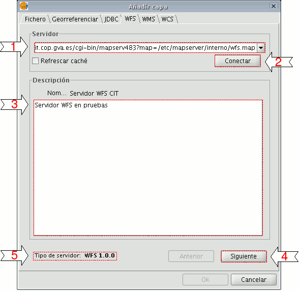
1. The pull-down menu shows a list of WFS servers (you can add a different server if you don’t find the one you want).
2. Click on “Connect”. gvSIG connects to the server.
3. and 4. When the connection is made, a welcome message from the server appears, if this has been configured. If no welcome message appears, you can check whether you have successfully connected to the server if the “Next” button is enabled.
5. The WFS version number that the server you have connected to is using is shown at the bottom of the box.
N.B. You can select the “Refresh cache” option which will search for information from the server in the local host. This will only work if the same server was used on a previous occasion.
Acceso al servicio
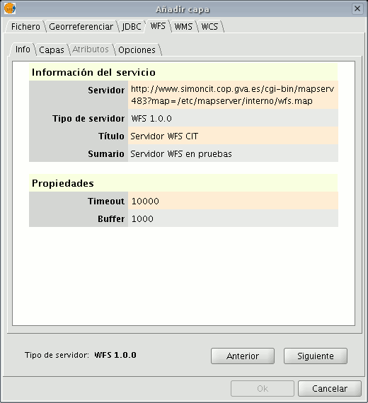
Click on “Next” to start configuring the new WFS layer.
When you have accessed the service, a new group of tabs appears. The first tab (“Information”) shows all the information about the server and about the request that is to be sent. This information is updated as more layers are selected.
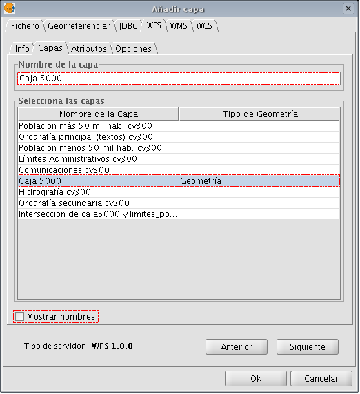
Selección de "Capas"
The “Layers” tab can be used to select the layer you wish to load. A two-column table appears in which the layer name and the geometry type are shown. As the geometry type is obtained by clicking on the layer (it needs to be obtained from the server), this column is completely blank at the start.
The “Show layer names” option shows the name of the layer as it is recognised by the server and not by its description, which is what appears in the table by default.
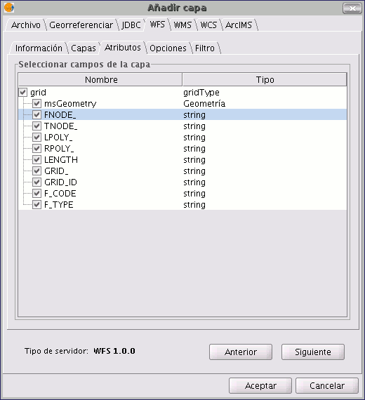
Selección de "Atributos"
The “Attributes” tab allows the fields (or attributes) of the selected layer to be selected. When the layer is loaded, only the fields that have been selected are retrieved.
To select the attributes, enable the check box which appears to their left.
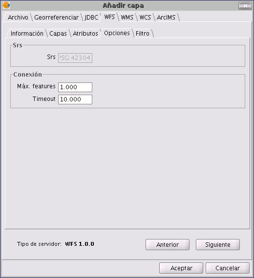
Pestaña "Opciones"
The "Options” tab shows information about user authentication and the connection. The “User” and “Password” fields are used in the WFS-T to be able to identify a user in the server so that writing operations can be carried out (not yet implemented).
The connection parameters are:
Number of features in the buffer, i.e. the maximum number of elements that can be downloaded.
Timeout. This is the length of time beyond which the connection is rejected as it is considered to be incorrect. If these parameters are very low, a correct request may not obtain a response.
The Spatial Reference System (SRS) is another important parameter. Although this cannot currently be changed, it is hoped that this will be possible in the future. In any case, gvSIG reprojects the loaded layer to the spatial system in the view.
Crear un filtro
You can use this tab to apply filters to your WFS layers. Click on the “Filters” tab in the window.
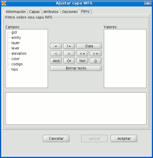
The “Fields” text box shows the layer’s attributes which can be used as a filter. Click on the selected field to see its values.
When the layer is loaded for the first time, the values in the column cannot be selected. However, if you have a filter sentence for the layer you can apply it in the filter text area and the filtered layer will be loaded directly.
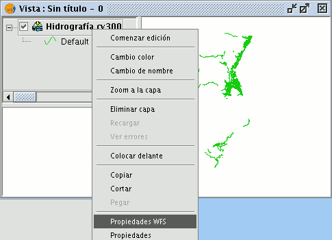
If you do not have a filter sentence, load the WFS layer into the ToC, then right click on the mouse and select the “WFS properties” option from the contextual menu.
To create the filter for the WFS layer, double click on the field you wish to use as a filter and it will appear in the bottom text area. Then click on the operator you wish to apply and finally select the value in the “Values” text area by double clicking on it.
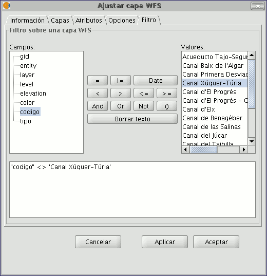
When you have created the required filter, click on “Ok” and it will be applied to the WFS layer.
Añadir una capa WFS a la vista
When all the parameters have been configured, click on “Ok”. The layer will be loaded into a gvSIG view.
Modificación de las propiedades de la capa
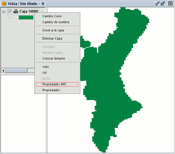
By right clicking on the layer, its contextual menu appears. If the “WFS Properties” option is selected, an option display opens (similar to the “Add layer” display). This can be used to select new attributes and other layers and change the layer’s properties.
Añadir capa a través del protocolo WMS
Introducción
Part of the gvSIG philosophy in its creation included the implementation of open standards for access to spatial data. Thus, gvSIG includes a WMS client which complies with the current OGC (Open Geospatial Consortium, http://www.opengeospatial.org) standard.
Conexión al servicio
Go to the "Add layer" window and then select the WMS tab.
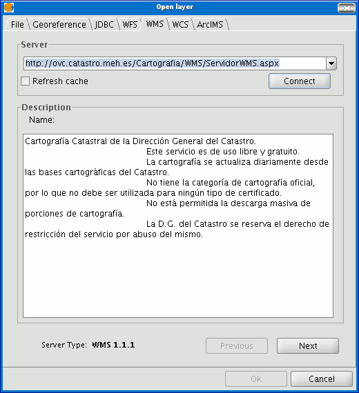
- The pull-down menu shows a list of WMS servers (you can add a different server if you don’t find the one you want).
- Click on “Connect”.
- and 4. When the connection is made, a welcome message from the server appears, if this has been configured. If no welcome message appears, you can check whether you have successfully connected to the server if the “Next” button is enabled.
- The WMS version number that the connection has been made to is shown at the bottom of the box.
Acceso al servicio
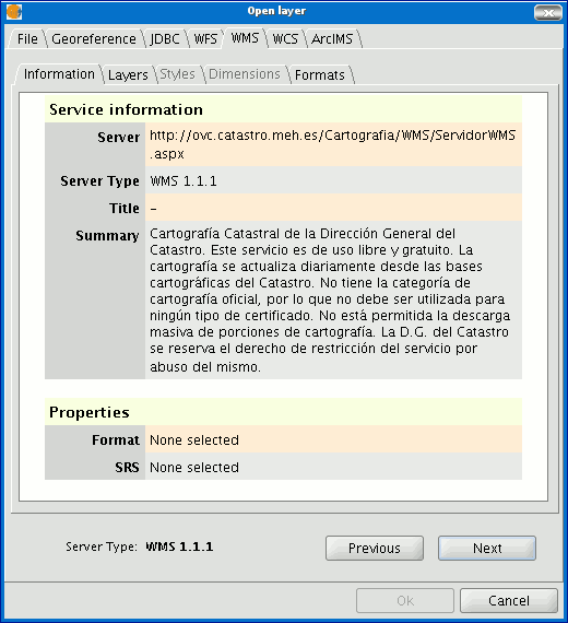
Click on “Next” to start configuring the new WMS layer.
When you have accessed the service, a new group of tabs appears.
The first tab in the adding a WMS layer wizard is the information tab. It summarises the current configuration of the WMS request (service information, formats, spatial systems, layers which make up the request, etc.). This tab is updated as the properties of its request are changed, added or deleted.
Selección de "Capas"
The wizard’s “Layers” tab shows the WMS server’s table of contents.

Select the layers you wish to add to your gvSIG view and click on “Add”. If you wish, you can choose a name for the layer in the “Layer name” field.
N.B. Several layers can be selected at the same time by holding down the “Control” key and left clicking on the mouse.
N.B. To obtain a layer description move the cursor over a layer and wait a few seconds. The information the server has about these layers is shown.
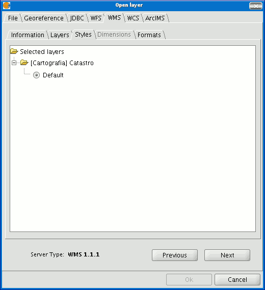
Selección de "Estilos" sobre las capas del servidor WMS
The “Styles” tab allows you to choose a display view for the selected layers. However, this is an optional property and the tab may be disabled because the server does not define styles for the selected layers.
Selección de valores para las "Dimensiones" de una capa WMS
The “Dimensions” tab helps to configure the value for the WMS layer dimensions. However, the dimensions property (like the styles property) is optional and may be disabled if the server does not specify dimensions for the selected layers.
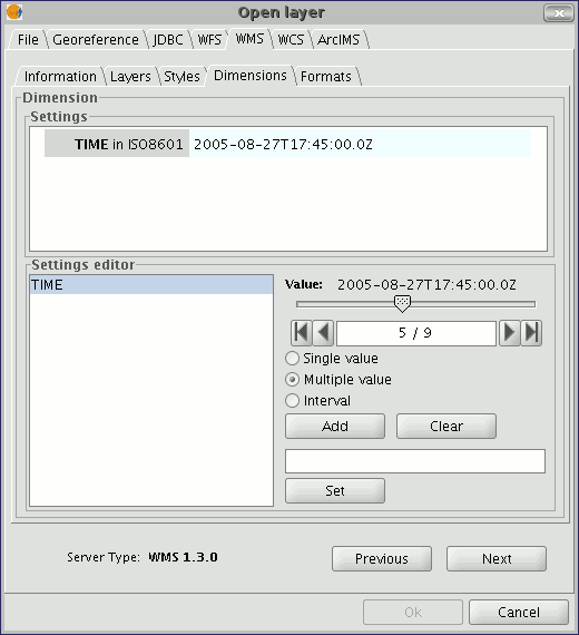
No dimension is configured by default. To add a dimension, select one from the “Settings editor” area in the list of dimensions. The controls in the bottom right-hand corner of the tab are enabled. Use the slider control to move through the list of values the server has defined for the selected dimension (for example “TIME” refers to the dates the different images were taken). You can move back to the beginning, one step back, one step forward or move to the end of the list using the navigation buttons which are located below the slider control. If you know the position of the value you require, you can simply write it in the text field and it will move automatically to this value.
Click on “Add” so that you can write the selected value in the text field and request it from the server.
gvSIG allows you to choose between:
Single value: Only one value is selected
Multiple value: The values will be added to the list in the order they are selected in
Interval: An initial value and then an end value are selected
When the expression for your dimension is complete, click on “Set” and the expression will appear in the information panel.
N.B. Although each layer can define its own dimensions, only one choice of value is permitted (single, multiple or interval) for each variable (e.g. for the TIME variable a different image date value cannot be chosen in each layer).
N.B. The server may come into conflict with the layer combination and the variable value you have chosen. Some of the layers you have chosen may not support your selected value. If this occurs, a server error message will appear.
N.B. You can personalise the expression in the text field. The dialogue box controls are only designed to make it easier to edit dimension expressions. If you wish you can edit the text field at any time.
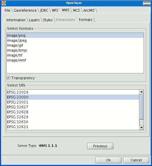
Selección de formato, sistema de coordenadas y/o transparencia
The “Formats” tab allows you to choose the image format the request will be made with, specify if you wish the server to hand in the image with a transparency (to superimpose the layer onto other layers the gvSIG view already contains) and also the spatial reference system (SRS) you require.
Añadir una capa WMS a la vista
As soon as the configuration is sufficient to place the request, the “Ok” button is enabled. If you click on this button, the new WMS layer will be added to the gvSIG view.
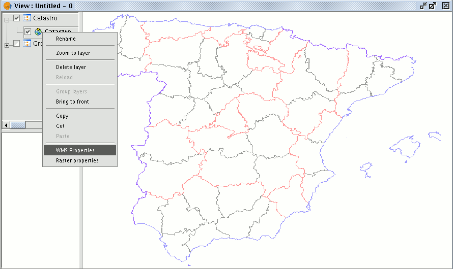
Modificación de las propiedades de una capa
Once the layer has been added its properties can be modified. To do so, go to the Table of contents in your gvSIG view and right click on the WMS layer you wish to modify. The contextual menu of layer operations appears. Select “WMS Properties”. The “Config WMS layer” dialogue window appears. This is similar to the wizard for creating the WMS layer and can be used to modify its configurations.
Añadir una capa a través del protocolo WCS
Introducción
The WCS (Web Coverage Service) is another of the OGC standards supported by gvSIG. The WCS is a coverage server. It is different from WMS as this standard defines a map as a representation of geographic information in the shape of a digital image file which can be shown on a computer screen. The map does not include its own data but WCS, however, does provide its own data, which can subsequently be analysed. WCS therefore allows raster data to be analysed just as WFS allows vector data to be analysed.
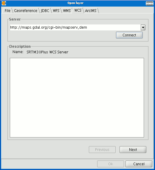
- The pull-down menu shows a list of WCS servers (you can add a different server if you don’t find the one you want).
- Click on “Connect”. gvSIG connects to the server.
- and 4. When the connection is made, a welcome message from the server appears, if this has been configured. If no welcome message appears, you can check whether you have successfully connected to the server if the “Next” button is enabled.
Acceso al servicio
Click on “Next” to start configuring the new WCS layer.
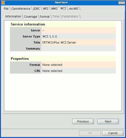
When you have accessed the service, a new group of tabs appears.
The first tab in the adding a WCS layer wizard is the information tab. It summarises the current configuration of the WCS request (service information, formats, spatial systems, layers which make up the request, etc.). This tab is updated as the properties of its request are changed, added or deleted.
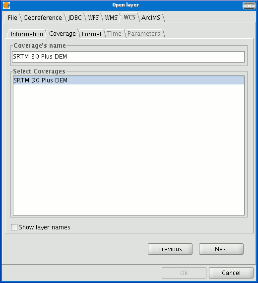
Selección de "Coberturas"
Select the coverage you wish to add to your gvSIG view. If you wish, you can choose a name for your layer in the “Coverage name” field.
Selección de "Formato"
You can choose the image format you wish to use to make the request and reference system (SRS) in the “Format” tab.
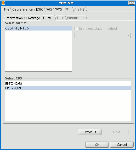
N.B. Tabs such as “Time” and “Parameters” are disabled in this case. Configuring these variables depends on the server chosen and the type of data it has access to.
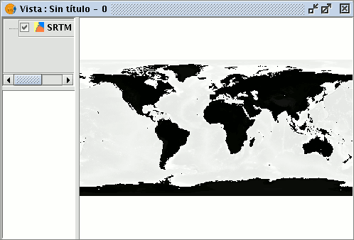
Añadir la capa WCS a la vista
As soon as the configuration is sufficient to place the request, the “Ok” button is enabled. If you click on this button, the new WCS layer will be added to the gvSIG view.
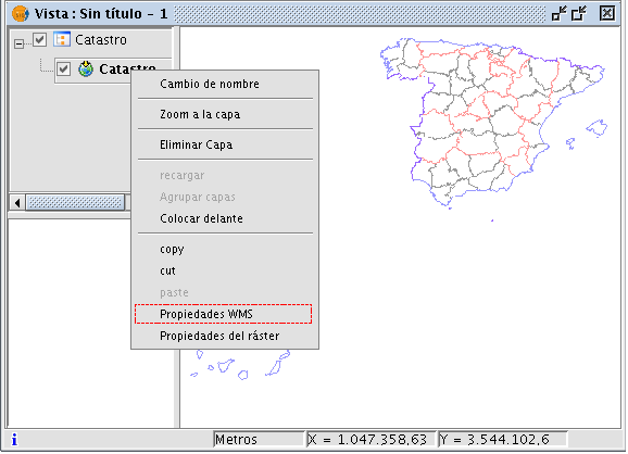
Modificación de las propiedades de una capa
Once the layer has been added its properties can be modified. To do so, go to the Table of contents in your gvSIG view and right click on the WCS layer you wish to modify. The contextual menu of layer operations appears. Select “WCS Properties”.
The “Config WCS layer” dialogue window appears. This is similar to the wizard for creating the WMS layer and can be used to modify your configurations.
Añadir una capa a traves del protocolo ArcIMS
Introducción a ArcIMS
In the proprietary software environment, ArcIMS (developed by Environmental Sciences Research Systems, ESRI) is probably the most widespread/popular widely used (Internet) cartographic server on the Internet thanks to the number of clients it supports (HTML, Java, ActiveX controls, ColdFusion...) and to its integration with other ESRI products. ArcIMS is currently one of the most important remote cartographic information providers. Although the protocol it uses does not comply with the Open Geospatial Consortium (because it was created long beforehand), the gvSIG team believes that offering support for ArcIMS is important.
Conexión a servicios de imágenes
The extension can access image services offered by an ArcIMS server. This means that, just like a WMS server, gvSIG can request a series of layers from a remote server and receive a view rendered by the server containing the requested layers in a specific coordinate system (reprojecting if necessary) and in specific dimensions. In addition to displaying geographic information, the extension allows you to request information about the layers for a particular point via the gvSIG standard information button.
ArcIMS is slightly different in its philosophy from WMS. In WMS, the request is normally made by independent layers whilst in ArcIMS the request is global.
The steps required to request a layer from an ArcIMS server and to request information for a particular point are listed below.
Carga de una capa a través de ArcIMS
Cargar una capa usando el protocolo arcims
Our example uses the ESRI ArcIMS server. Its URL is http://www.geographynetwork.com. This is the address a web browser requires to access the HTML visual display unit.
Before loading a layer from this server, the datum WGS84 in geodesic coordinates (code 4326) has to be set up previously as the view’s spatial system.
Conexión al servidor
If the extension is loaded correctly, a new ArcIMS data source will appear in the “Add layer” dialogue box.
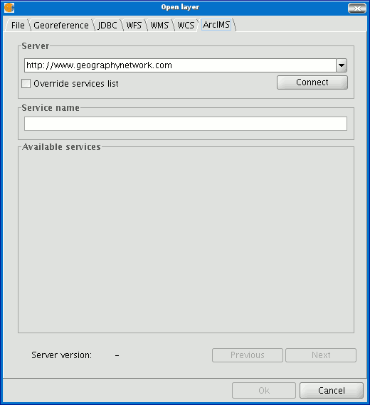
Adding a new layer to the view
If the server has a standard configuration, simply indicate its address. gvSIG will try to find the servlet’s full address.1 If the servlet has a different path, you will have to write it into the dialogue box.
When the connection has successfully been made, the server version, its compilation number and a list of image and geometry services available are shown.
The service can be selected from the list or can be written in directly.
Finally, if the “Override service list” check box is enabled, gvSIG will delete any catalogue that has already been downloaded and will request them again from the server.
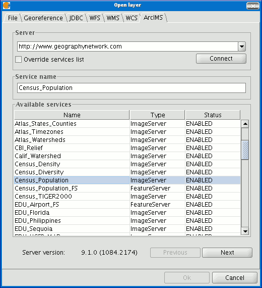
List of services available
Acceso al servicio
The next step is to select the ImageServer type service required by double clicking or selecting it and clicking on "Next". The dialogue box changes and an interface with two tabs appears (fig. 3). The first tab shows the metainformation given by the server about the service’s geographic limits, the acronym of the language it has been written in, units of measurement, etc. It is a good idea to find out if a coordinate system has been defined in the service (using EPSG codes) as this can directly influence the requests made to the server, as Figure 3 shows.
N.B. If no coordinate system has been defined in the service, the extension will assume that it is the same coordinate system as the one we have defined for the view.
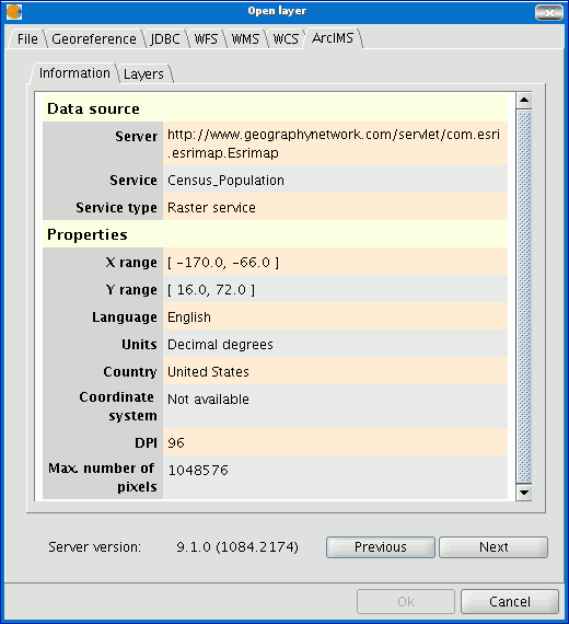
Figure 3: Metadata from the ArcIMS server
We can continue by clicking on "Next" or return to the previous dialogue by clicking on "Change service”.
Selección de capas
The last dialogue box is the layer selection. We can define a name for the gvSIG layer or leave the default value (the service name) in this window. A box appears below with a list of the service layers in tree form. When the mouse is moved over the layers, information about these layers appears: extension, scale ranges, type of layer (raster or vector image) and if it is visible by default in the service (fig. 4).
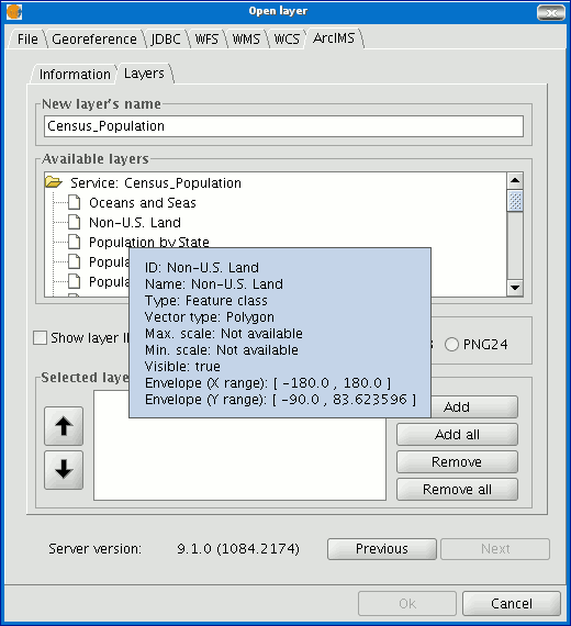
Figure 4: Metadata from a service layer
We can view each layer’s ID via the “Show layer ID” check box. This check box is useful when there are layers whose descriptor is repeated. Therefore, the only way to distinguish between them is via an ID, which will always be unique. A combo box is also available to select the image format we wish to use to download the images. We can choose JPG format if our service works with raster images or one of the other remaining formats if we want the service to have a transparent background.
N.B. The transparency in 24-bit PNG images is not correctly displayed in gvSIG 0.6. This type of files will be supported in gvSIG 1.0.
The box with the layers selected for the service appears below. If you wish, you can add just some of the service layers and also reorganise them. This makes the service view totally personalised.
N.B. The configuration cannot be accepted until a layer has been added.
N.B. Multiple selections of service layers can be made by using the Control and CAPS keys.
Añadir la capa a la vista
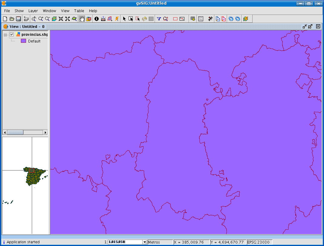
When the “Ok” button in the dialogue box is pressed, a new layer appears in the view (fig. 5). If no layer has been added previously, the extension of the ArcIMS layer is shown, as per the standard gvSIG procedure.
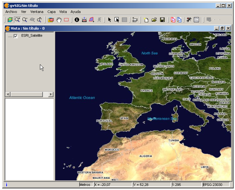
Figure 5: ArcIMS layer added to the gvSIG view.
It must be remembered that when the layer extension is shown, the layers that make up the chosen configuration may not appear and a blank or transparent image appears instead. If this occurs, use the scale control dialogue box (V. Information about scale limits section).
Consideraciones a tener en cuenta respecto a los sistemas de referencia
An ArcIMS server does not define the spatial reference systems it supports as opposed to the WMS specification. This means that a priori we do not have a list of EPSG codes that the map server can reproject. In short, ArcIMS can reproject to any coordinate system and leaves the responsibility of how the projections are used to the client.
Therefore, if our gvSIG view is defined in ED50 UTM zone 30 (EPSG:23030) and we request a global coverage service (stored for example in the geographic coordinates WGS84, which correspond to code 4326) the server will not be able to reproject the data correctly because we are using global coverage for a projection of a specific area of the Earth.
However, the procedure can be carried out in reverse. If we have a view in geographic coordinates (and thus global coverage), services defined in any coordinate system can be requested because the server will be able to transform the coordinates correctly.
In short, requests to the ArcIMS server must be made in the view's coordinate system and they cannot be requested in another coordinated system.
Moreover, as we mentioned above, if an ArcIMS server does not offer information about the coordinate system its data is in, the user will be responsible for setting up the correct coordinate system in the gvSIG view. Thus, if a user with a view in UTM adds a layer which is in geographic coordinates (even though the server does not show it), the service will be added correctly but will take the view to the geographic coordinates domain (in sexagesimal degrees).
An additional effect is that if the view uses different units of measurement from the server, the scale will not be shown correctly.
Modificación de las propiedades de la capa
The layers requested from the server can be modified via a dialogue box, which can be accessed from the layer’s contextual menu (fig. 6) just like the WMS layers. This dialogue box is similar to the box used to load the layer, apart from the fact that the service cannot be changed.
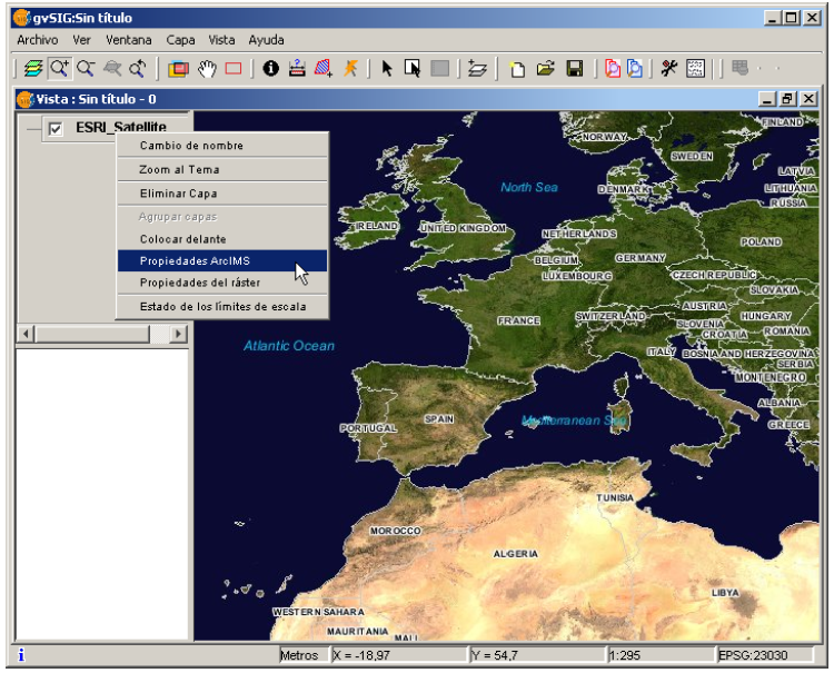
Figure 6: Properties of the ArcIMS layer
Información sobre los límites de escala
The extension allows us to consult the layers' scale limits which make up the requested service via a dialogue box which can be maintained in the view during the session (fig. 7). This window shows the layers on the vertical axis and the different scale denominators on the horizontal axis via a logarithmic scale. This box is small on screen but can be enlarged to improve the difference between the scales.
The vector layers, raster layers and the layers that can be seen on the current scale (marked with a vertical line) in a darker colour and the layers we cannot see above or below the current scale are differentiated by different coloured bars (described in the window legend).
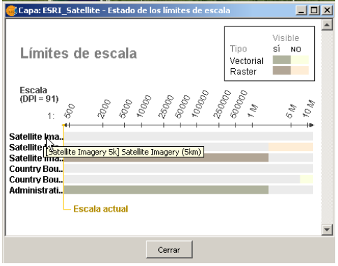
Figure 7: Scale limits status
Consulta de información de atributos
Attribute information requests about the elements for a particular point is one of gvSIG’s standard tools. Its functionality is also supported by the extension.
The WMS specification allows information about several layers to be requested from the server in one single query. This is different in ArcIMS. We need to make one server request per layer required.
This means that no requests for unloaded layers or unseen layers that are not visible on the current scale or layers whose extension is outside the view will be made. Even if all these layers are filtered, the information request usually takes longer than is desirable because of this intrinsic feature of ArcIMS.
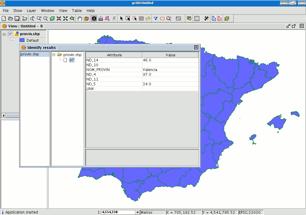
When all the request responses have been recovered, the standard gvSIG attribute information dialogue appears with each of the layers (LAYER) which return information as a tree. If we click on a layer, its name and ID appear on the right (fig. 8).
Under this node, if we are talking about a vector layer, all the records or geometric elements the server has responded to appear, and give each one their corresponding attributes (FIELDS).
If it is a raster layer, such as an orthoimage or a digital terrain model, it returns the values for each of the bands (BAND) in the requested pixel colour, instead of records.

Figure 8: Displaying attribute information
Conexión a servicios de geometrías
The extension allows access to both ArcIMS image services and geometry services (Feature Services). This means that a server can be connected to and geometric entities (points, lines and polygons) and their attributes obtained. This is not dissimilar to WFS service access.
However, the variety of existing geometry services is much lower than the variety in the image server. There are two main reasons for this. On one hand, providing the public with vector cartography implies security problems because many bodies only want to offer the general public views and images. The vector data becomes either an internal product or must be paid for. On the other hand, this type of services generate much more traffic on the network and in the case of basic information servers could become a problem.
Carga de una capa de geometrías
Loading a geometry layer is practically the same procedure as loading the image server as mentioned above (Accessing the service section and the following sections). In this case, the number of layers to be selected must be taken into account. If we wish to download all the layers offered by the service the response time will be very high.
The only difference between loading an image layer is that in this case we can choose whether we wish the layers to be downloaded as a group via a check box. This is useful for processing the vector layers as one layer when it needs to be moved and activated in the table of contents.
Unlike the image service, in which all the service’s layers appear as one unique layer in the gvSIG view, in this case each layer is downloaded separately and appears in the view grouped under the name defined in the connection dialogue.
Simbología en ArcIMS
Cartography symbols are configured in the server in one AXL extension file for both geometry and image services. We can divide symbol definition into two parts. On one hand, we can talk about the definition of the symbols themselves, i.e. how a geometric element, such as a line or polygon, should be presented. On the other hand, we can talk about the distribution of these symbols according to the cartographic display scale or to a specific theme attribute.
In ArcIMS terminology symbols are different from legends (SYMBOLS and RENDERERS).
Símbolos
There are various types of symbols: raster fill symbols, gradient fill symbols, simple line symbol, etc. The extension adapts the majority of the symbols generated by ArcIMS. Table 1 shows the ArcIMS symbols and indicates whether they are supported by gvSIG.
| Label | Description | Supported |
|---|---|---|
| CALLOUTMARKERSYMBOL | Balloon-type label | NO |
| CHARTSYMBOL | Pie chart symbol | NO |
| GRADIENTFILLSYMBOL | Fill in with gradient | NO |
| RASTERFILLSYMBOL | Fill with raster pattern | YES |
| RASTERMARKERSYMBOL | Point symbol using pictogram | YES |
| RASTERSHIELDSYMBOL | Customised point symbol for US roads | NO |
| SIMPLELINESYMBOL | Simple line | YES |
| SIMPLEMARKERSYMBOL | Point | YES |
| SIMPLEPOLYGONSYMBOL | Polygon | YES |
| SHIELDSYMBOL | Point symbol for US roads | NO |
| TEXTMARKERSYMBOL | Static text symbol | NO |
| TEXTSYMBOL | Static text symbol | YES |
| TRUETYPEMARKERSYMBOL | Symbol using TrueType font character | NO |
Table 1: ArcXML symbol definition labels
In general, the most common symbols have been successfully “transferred”. Some of the symbols cannot be obtained directly from gvSIG (at least in the current version), such as the raster fill symbol or they need to be “adjusted” such as the different types of lines. This means that a raster fill symbol is not a symbol that can be defined by the gvSIG user interface, but it can be defined by programming.
Leyendas
gvSIG supports the most common types of legends: unique value and range and value themes as well as the scale-range control over the whole layer. ArcIMS goes much further in its configuration. It can generate much more complicated legends in which symbols can be grouped together, scale-range controls can be established for labels and symbols and different labelling based on an attribute can be shown (as though it were a value theme for labelling).
This group of legends can generate very complex symbols for a layer in the end. The current implementation status of the gvSIG symbols needs to be simplified to reach a compromise to recover the symbols that best represent the layer as a whole.
| Label | Description |
|---|---|
| GROUPRENDERER | Legend which groups others together |
| SCALEDEPENDENTRENDERER | Scale dependent legend |
| SIMPLELABELRENDERER | Labelling layer legend |
| SIMPLERENDERER | Unique value layer legend |
| VALUEMAPRENDERER | Value and range themes |
| VALUEMAPLABELRENDERER | Labelling themes |
Table 2: ArcXML legend definition labels
When a GROUPRENDERER is found, the symbol ArcIMS draws first is always chosen. Thus, in the case of the typical motorway symbol for which a thick red line is drawn and a thinner yellow line is drawn over it, gvSIG will only show the red line with its specific thickness.
If a scale dependent legend is discovered during a symbol analysis, this is always chosen. If more than one is discovered, the one with the greatest detail is chosen. For example, in ArcIMS we can have a layer with simple road symbols (only main roads are drawn) on a 1:250000 scale and based on this a different theme is shown with all types of roads (paths, tracks, roads, etc.). In this case, gvSIG will show this last theme as it is the most detailed.
If a labelling legend is discovered during a symbol analysis, it will be saved in a different place and will be assigned to the selected definitive legend. In the case of the VALUEMAPLABELRENDERER label, only the legend of the first processed value will be obtained as a label symbol. The rest will be rejected.
In short, it is obvious that the failure to adapt the legends for gvSIG is a simplification process in which different legend and symbol definitions must be rejected to obtain a legend which is similar to the original as far as possible. It is to be expected that the gvSIG symbol definition will improve considerably so that it can support a larger group of cases in the future.
Trabajo con la capa
Working with the layer is similar to any other vector layer, as long as we remember that access times may be relatively high. The layer attribute table can be consulted, in which case the records will be downloaded successively as we display them.
If we wish to change the table symbols to show a unique value or range theme we must wait as gvSIG requests the complete table for these operations. On the other hand, the downloading of attributes is only carried out once per layer and session and therefore, this wait only occurs in the first operation.
In general, if our ArcIMS server is in an Intranet, it will be relatively fast to handle, but if we wish to access remote services we may be faced with considerable response times.
The main feature to bear in mind when working with an ArcIMS vector layer is that the geometries available at any given time are only the ones displayed. This is because we can connect to huge layers but only the visible geometries are downloaded. As far as gvSIG is concerned, the geometries shown on the screen are the only ones available and thus, if we export the view to a shapefile for example, are only a part of the layer.
Finally, we need to remember that to speed up the geometry downloads they are simplified to the viewing scale in use at any given time. This drastically reduces the amount of information downloaded as only the geometries that can actually be "drawn" are displayed in the view.
Loading a geometry layer is practically the same procedure as loading the image server as mentioned above (Accessing the service section and the following sections). In this case, the number of layers to be selected must be taken into account. If we wish to download all the layers offered by the service the response time will be very high.
Unlike the image service, in which all the service’s layers appear as one unique layer in the gvSIG view, in this case each layer is downloaded separately and appear in the view grouped under the name defined in the connection dialogue.
After a few seconds the layers appear individually but are grouped under a layer with the name we have defined for it.
The layer symbols are established at random. A pending feature is to recover the service symbols and configure them by default so that gvSIG can display the cartography as similarly as possible to how it was established by the service administrator.
Añadir ortofotos a traves del protocolo ECWP
If you wish to add an orthophoto to gvSIG using the ECWP protocol, first open a view and click on the “Add layer” button.

Click on the “Add” button in the dialogue box. A file browser window appears.
Choose the “gvSIG Image Driver” option from the “Files of type” pull-down menu.
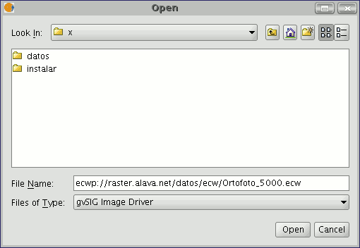
Write the URL of the file you wish to load as follows in “File name”:
ecwp://server address/path of the file you wish to add.
For example:
ecwp://raster.alava.net/datos/ecw/Ortofoto_5000.ecw
ecwp://earthetc.com/images/geodetic/world/MOD09A1.interpol.cyl.retouched.topo.bathymetry.ecw
When you have input the data, click on “Open”.
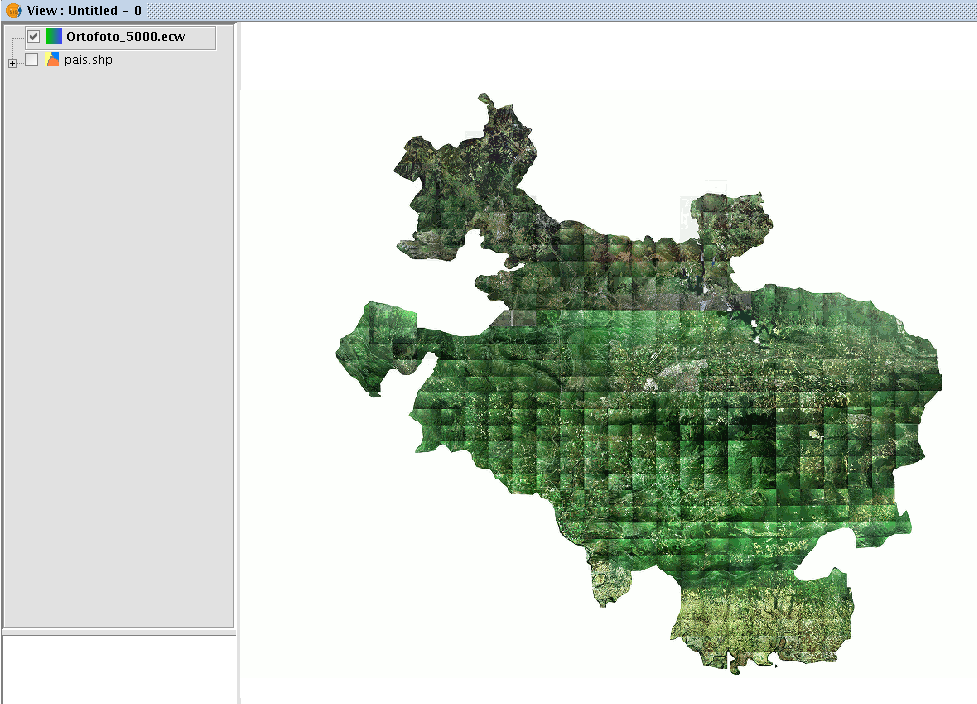
The orthophoto will be added to the layer list.
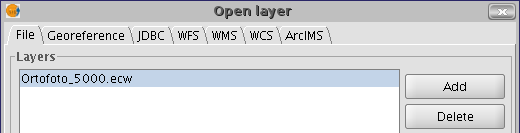
Select the new added layer and click on “Ok”.
The image will be added to the view.
Crear una nueva capa
Introducción
gvSIG can create a new layer in the following formats: shp, dxf and postgis.
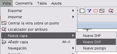
The tool can be accessed from the “View / New Layer” menu.
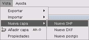
Crear nuevo SHP
Select the “New SHP” option opens the wizard which will help you create the new layer.
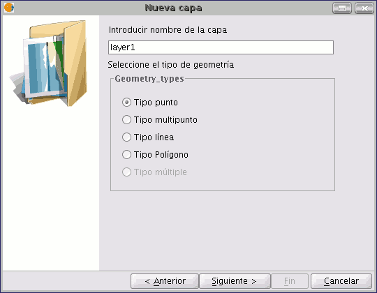
The first window of the wizard allows you to choose the name you wish the new .shp file to appear with in the ToC, in addition to the geometry type associated with it.
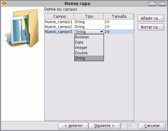
The second window of the wizard allows you to add all the fields you wish to the attribute table associated with the layer and to define some of the properties of these fields.
To add fields to the table, click on “Add field”. One field is added every time you click on this button.
If you wish to delete any of the fields created, simply select the field and click on the “Delete Field” button. You can edit the rest of the properties from the attribute table in which the fields are defined.
Field name: Place the cursor over the field name (“New field” by default) and write the new name. The maximum number of characters allowed for the field name is 10.
- Field type: Place the cursor over any of the files in the “Type” field. A pull-down menu appears in which the type of field you wish to create can be selected.
- BOOLEAN: Boolean type data admits “true” or “false” values.
- DATE: This allows you to create a field which includes dates. The maximum number of characters allowed is 8.
- INTEGER and DOUBLE are two number type fields. The former is for whole numbers and the latter for decimal values.
- STRING: This is an alphanumeric field type. The maximum number of characters allowed is 254.
Field length: This allows you to set the maximum number of characters for the field created (at present, this only applies to String-type fields).
Once the structure of the table associated with the shape file has been determined, click on “Next”.

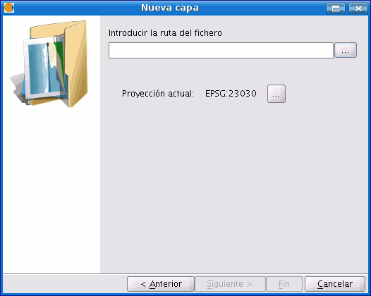
You can save the file in the new window and choose the Reference System for the view the new layer is going to be inserted into by clicking on the button to the right of “Current Projection”.
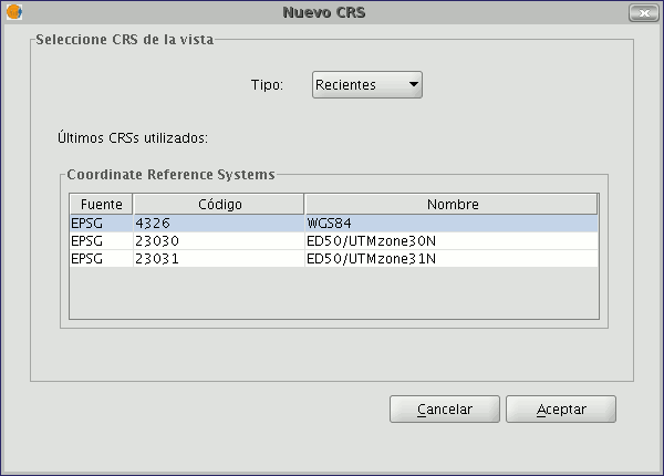
If other layers have been inserted in the view, this button will be disabled since the view already has a selected reference system.
To save the new layer, indicate the file path to save the file in the text box.
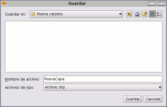
You can also open the search dialogue box to select the file path the new shape file will be saved in. To do so, click on the button to the right of the text box. Write the name for the new layer (remember that this name will appear in the source file of the shape file and that it may be different to the name which appears in the ToC) and click on the “Save” button.
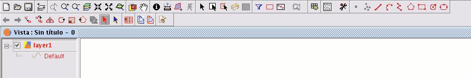
When you have finished creating a new SHP file, it will be added to the ToC.
In addition, the editing tools will be activated to allow you to create the elements of the new layer.
Crear un nuevo DXF
The procedure to create a new DXF file is similar to that used to create a new SHP file, as described in the previous section. This tool can be accessed from the “View/New layer/New dxf” menu.
If this tool is selected, the wizard will open a window allowing you to select a path for the file which is going to create a reference system for the view.
Crear un nuevo PostGis
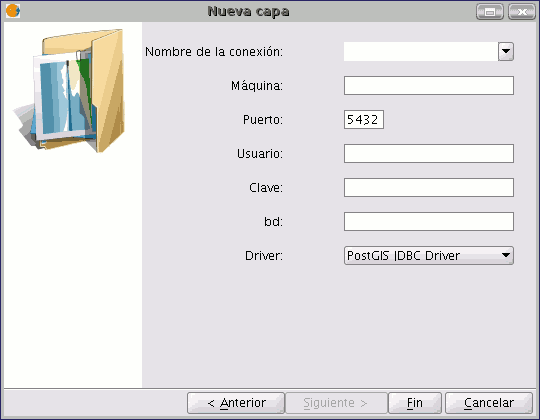
If you wish to create a new PostGIS file, go to the menu “View/New layer/New PostGIS”.
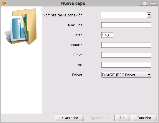
The initial steps to create a new PostGIS file are similar to those followed in the section on creating a new Shape file.
The difference lies in the way the new layer is saved, as this is entered into a PostGIS data base.
Fill in the fields which apply to your connection and click on “Finish”.
Añadir capa de Eventos
Introducción
A new layer can be created from a table in gvSIG by using “Add event layer”.
There are two ways to do this: you can add a table to the project or you can work with a table associated with one of the layers in the view in which you are working at a particular time.
Añadir capa de eventos desde una tabla nueva
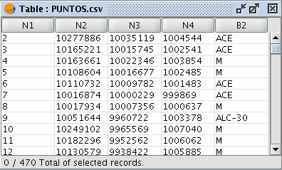
Firstly, the table needs to be loaded. To do so, go to the gvSIG “Project manager” and select "Tables" in document types. Then click on "New".
A search dialogue opens to add the table you require. Click on "Add".
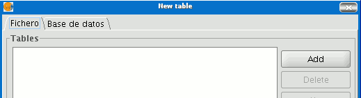
A dialogue box appears in which you can choose two types of data sources: dbf and csv.
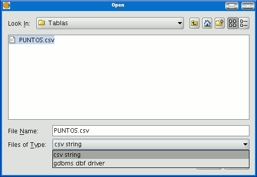
When you have found the table you require, select it and click on “Open”.
gvSIG automatically returns to the "New table" window and adds the table you require to create the event layer in the text box.
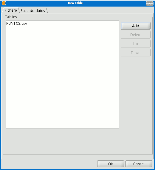
Click on “Ok” to finish the process.
When the table has been added, a view must be active to create its corresponding event layer and load it. If no view is active, you can return to the “Project manager” and add one or create a new blank one. When you have activated this view, go to the “Add event layer” by using the corresponding button in the tool bar:

A window with three pull-down menu bars appears.
We can select the table we need to add the new layer from the first pull-down menu bar.
Then, we can select the table fields which will become the X and Y values.
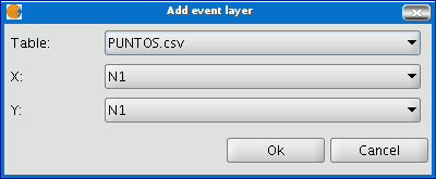
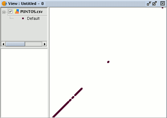
If you click on “Ok”, a new points layer will appear based on the coordinates contained in the initial table.
Añadir capa de eventos desde una tabla asociada a una capa de la vista
If you wish to work with a table associated to the layers in the view, you will firstly have to activate the attribute table of this layer. To do so, click on the following button in the tool bar:

If you click on “Add event layer”

you will see that the table has been added.
Propiedades de la capa
Introducción
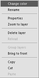
You can access the active layer's properties from its contextual menu (right click on the layer).
Capa vectorial
Cambiar el color de una capa añadida
Go to the layer’s contextual menu and click on the “Change colour” option. A window opens in which you can select the colour you wish to view the layer with.
There are three ways to select the colour depending on the window tab you select.
Swatches
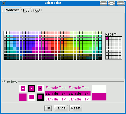
Selecting the colour from the “Swatches” tab is relatively easy. Place the mouse pointer over the desired colour on the palette and left click.
The colours you have used recently appear in the "Recent” palette.
HSB
A colour can be defined by its hue, brightness and saturation values. Any colour can be identified by values of these three variables. Black is obtained when there is an absence of light. Grey is obtained when the saturation is low (high light interference or mixture). White is the brightest colour of the greys (maximum frequency of different length waves).
This colour representation model is called HSB (Hue, Saturation, Brightness).
gvSIG has a colour selection window based on the HSB and RGB system which allows colour to be selected via HSB attributes and also obtain RGB values to reproduce them on the screen.
The following table shows the Hue variations which are represented on the horizontal axis of the square. The Saturation variations are represented on the vertical axis and the Brightness variations are shown on the side bar.
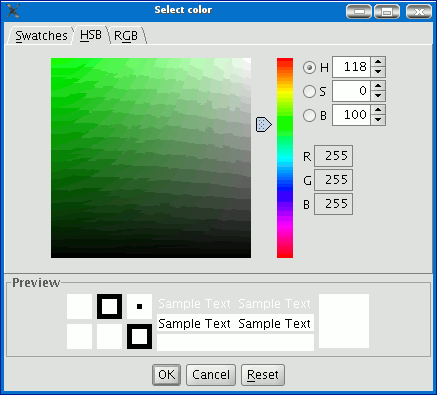
You can set one of the colour values by clicking on the corresponding check box. Click on the square area to define the values for the other 2 parameters. Slide the horizontal bar to set the value for the parameter marked with the check box.
When you have defined the colour you require, click on “Ok”.
RGB
RGB colour uses an additive model, in which the primary colours (red, green and blue) are combined to make other colours.
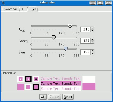
In this case, each primary colour is coded with a byte, so that each value is in a natural numbers [0, 255] interval. Thus, the RGB combination for black is R=0, G=0, B=0 and R=255, G=255, B=255 for white.
Cambiar el nombre a una capa añadida
If you wish to rename the selected layer, right click on the layer and go to the "Rename" option.
A new window appears:
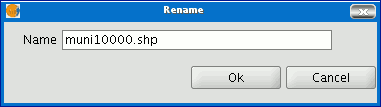
Write the new name in the text field and click on “Ok”.
N.B.: When you do this, the layer name changes in the ToC, but the file name is not changed.
Propiedades
Introducción
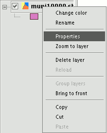
Right click on the selected layer in the ToC to access the properties window.

When you click on the “Properties” option, a new dialogue box opens. This can be used to edit some properties.
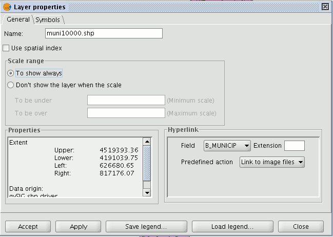
The layer name can be changed by writing the new name in the text field in the “General” tab.
Usar índice espacial
If you mark the “Use spatial index” check box, a spatial index will be created which makes the layer loaded in the view appear more quickly. This is because the view is loaded using this index.
If there are write permissions, a .qix file is created with the same name as the layer it is associated with in the layer’s original directory. If there are no write permissions, the file will be created in the user’s temporary file directory.
Rango de escalas
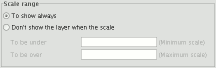
A viewing scale range (maximum and minimum) can be set in the properties window.
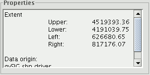
Resumen de las propiedades de las capa y su ruta de localización
The file extension and path are shown in the actual properties section.
Crear un hiperenlace en una capa
A link can be set up between a text, html or image file and a layer element in the properties window.
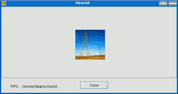
To provide a better idea of how the tool works, let us look at the following example. The aim is to link the image torreelectrica.jpg to a specific element:
Activate the view in the ToC.
Change the layer into editing mode (“Layer” menu then “Start edition”).
Open the table of attributes and edit the record you wish to create the link to. Write the path of the file you wish to link without its extension. Press “Enter” to save the modification made in the table.
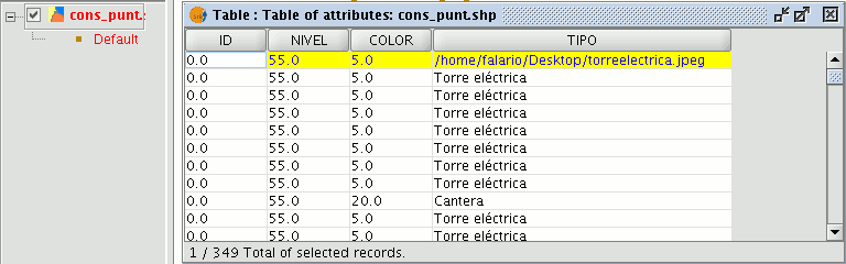
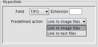
Go to the “Hyperlink” table in the layer properties window and select the field the record is located in which will be used to create the hyperlink. Write the extension of the file you wish to link and whether it is an image file (gif, jpg, png) or a text file (at present gvSIG can only link plain text files (txt, rtf...). Html files can also be linked. In this case, write html in the “Extension” text box and select “Link to text files”.
When all the requirements have been selected, click on “Apply” and then on “Ok”.
Then go the view tool bar and click on the hyperlink button.

Select the view element that corresponds to the record which has the associated link and place the cursor over it. Click on the element. A window appears with the linked file.
Editor de leyendas
Introducción
This tool can be used to carry out theme mapping relatively easily.
To symbolise or represent the element data or variables in a layer, you can choose the most suitable colour, pattern, etc. for each one.
Go to the “Properties” menu (right click on the layer) to edit the legend symbol properties.
A new window appears. Click on the “Symbols” tab.

Use this tab to define the legend type you wish to use to represent the layer data more specifically.
You can choose between the following:
Unique symbols: This is gvSIG’s default legend type and represents all the elements of a layer using the same symbol. It is useful if you need to show the location of a layer over and above any of its other attributes.
Unique values: Each record can be represented by a unique symbol according to the value it has in a particular field in the table of attributes. It is the most effective method to show categorical data, such as towns, types of land, etc.
Intervals: This type of legend represents the layer elements using a range of colours. The intervals or graduated colours are mainly used to represent numerical data which increase progressively or have a range of values, such as population, temperature, etc.
Labelling: Texts or labels can be automatically added to the view according to the values each element has in a particular field in its table of attributes.
The options shown in the symbols menu vary according to the type of layer (point, line or polygon layer).
The options available for a polygon layer, which has the most configuration tools, are shown below.
A legend can be saved or loaded (recovered) at any time.
Símbolo único
The following symbol configuration options are available:
Fill: Allows the fill colour to be selected.
Fill type: Allows the fill pattern to be selected.
Line: Allows the line colour to be selected.
Line style: Allows the style of the line to be selected.
Synchronising line and fill colours.
Line width: Allows the width of the line to be defined.
Transparency: Gives the elements a degree of transparency so that polygon layers can be superimposed and yet still viewed.
In point-type shape layers you can use the “Unique symbol” option in the “Symbols” tab to define the symbol type, the colour and point size you wish this layer to be displayed with.
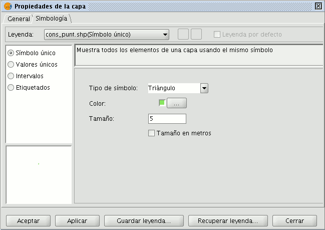
· Click on the “Symbol type” pull-down menu and select the symbol you wish the layer to be displayed with. Select the colour and set the size of the symbol you have chosen.
Click on “Apply” to see a preview of the set configuration.
Click on “Ok” if you wish to make this configuration permanent.
Click on the “Symbol type” pull-down menu and select the symbol you wish the layer to be displayed with. Select the colour and set the size of the symbol you have chosen.
Click on “Apply” to see a preview of the set configuration.
Click on “Ok” if you wish to make this configuration permanent.
Valores únicos
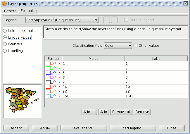
The following symbol configuration options are available:
Classification field: A pull-down menu appears in which you can select the layer’s table of attributes’ field which contains the data to be sorted.
Add all/Add: Once you have selected the “Classification field”, click on the “Add all” button to see all the different values. These values have all been assigned a different symbol (colour). Click on these symbols to modify them. By default, the label (the name which appears in the legend) is similar to the value it has in the field. You can include new values to the list by pressing the “Add” button.
Remove all/Remove: This allows all (Remove all) or some (Remove) of the elements in the legend to be removed.
Labels: Left click on any of the “Label” “cells” to modify the name they will have in the legend.
Intervalos
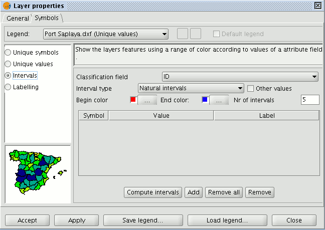
Classification field: A pull-down menu appears in which you can select the layer’s table of attributes’ field, which contains the data to be sorted. The field must be numerical because this is a gradual classification (by ranges of values).
Number of Intervals: This must indicate the number of ranges or intervals that define its classification.
Start colour and End colour: Select the colours to be graduated. The start colour is for the lowest values and the end colour is for the highest values.
Computing intervals: When you have defined the previous options, click on the “Compute intervals” button to see the legend’s end result. The symbols and the labels which appear by default can be modified by clicking on them, as in the previous cases.
Add: New ranges can be added to the computed intervals.
Remove all / Remove: This allows all (Remove all) or some (Remove) of the elements in the legend to be removed.
- Type of intervals: From gvSIG version 0.4 onwards, you can specify the interval type you wish to divide the information into in order to represent it. You can choose between the following options:
- Equal intervals: The number of intervals are specified and the sample is divided into this number of equal intervals.
- Natural intervals: The number of intervals is specified and the sample is divided into this number of intervals according to the Jenk method of optimising the natural breaks for the intervals.
- Quantile intervals: The number of intervals is specified and the sample is divided into this number of intervals but the values are grouped together according to their order number.
Etiquetado
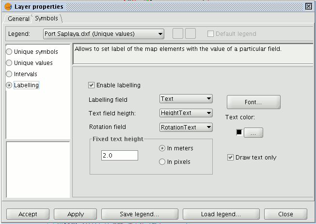
Enable labelling: Activate the check box to make the labelling visible in the view.
Labelling field: This is a pull-down menu which allows you to choose the layer’s table of attributes’ field, which contains the values to be shown as labels.
Text height field: This allows you to choose the layer’s table of attributes field which contains the values to be used for the label height.
Text rotation field: This allows you to choose the table of attributes field which indicates the label rotation angle.
Text colour: Allows the text colour to be selected.
Font: Allows the type of font to be selected.
Constant text height: Select the units (metres or pixels) and the text size. If you select “pixels”, the apparent text size will remain constant, even if you change the viewing scale; if you select “metres”, the text height on the display will vary according to the scale you are working in but will remain constant in geographic units.
Capa raster
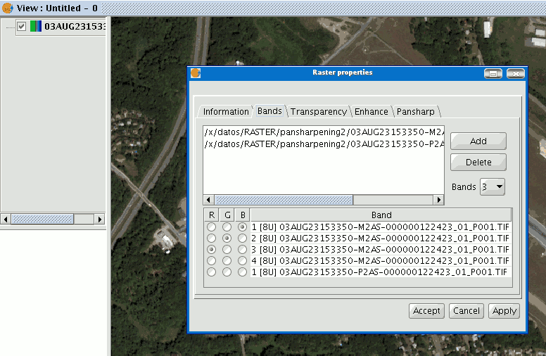
Propiedades del raster
Right click on a raster layer and select the "Raster properties" option. This opens a menu in which we can carry out various operations on the raster layer.
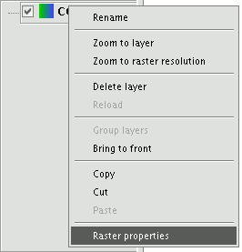
This menu is divided into five tabs:
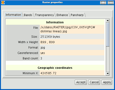
Information: Provides general information about the raster layer, the file path, the number of bands, the pixel dimensions, the file format, the data type and the geographic coordinates of the corners.
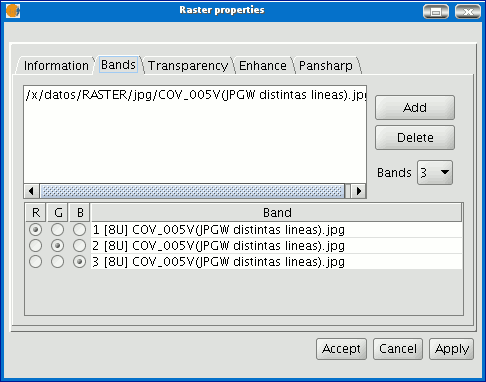
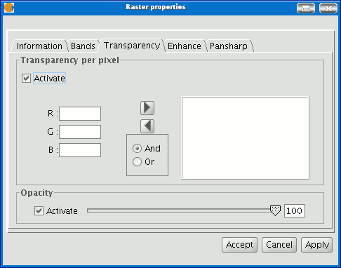
Bands: Provides tools to change the mode in which each image band is viewed. Transparency: Provides tools to change the transparency levels that can be applied to a raster layer.
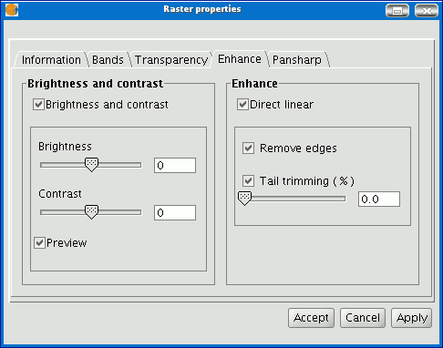
Enhance: Provides a tool to enhance the raster layer. Pansharpening: Provides a tool to increase the satellite image resolution if the panchromatic band for these images is available.
In the “Bands” tab you can make compositions using the different bands in a raster image. You can also add more bands from other files. This is useful when working with Landsat-type images, in which each band is delivered in a different file.
In addition to the “Transparency” option in gvSIg version 0.3, which is now called “opacity”, and which indicates the "occlusion” percentage of this layer over the previous ones, there is now a transparency option which allows the indicated colour groups (RGB) to be completely transparent. This is very useful to eliminate visual artefacts as a result of missing data in orthophotos or satellite images and to remove borders in an image mosaic.
To access the options, click on the corresponding “Activate” check boxes.
The “Enhance” tab can be used to modify the image brightness, contrast and enhancement. This last option is essential to be able to view 16-bits per band images correctly.
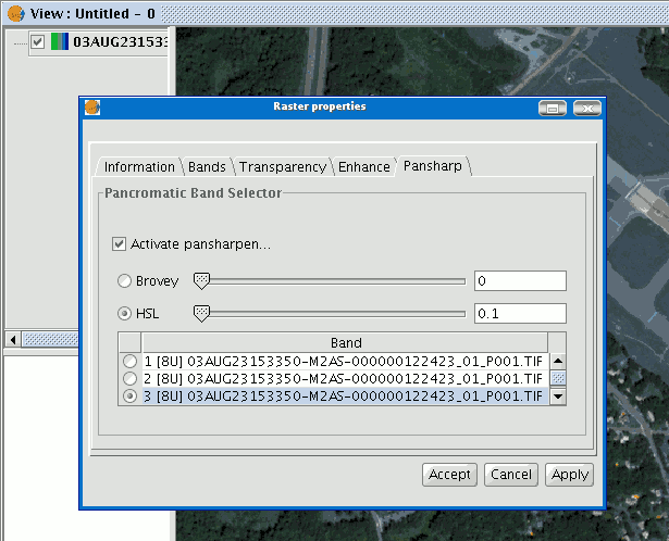
The “Pansharpening” tab can be used to increase the resolution of satellite images if the panchromatic band for these images is available. N.B.: If the image bands are in different files, they must be added to the layer using the “Bands” tab.
Use the “Bands” tab to find the best band combination for the view. In this section, you can load the image which corresponds to the panchromatic band but you must not select it to be visualised.
When the bands have been loaded, you can carry out the pansharpening. Go to the “Pansharpening” tab and activate it by clicking on the “Activate Pansharpening” check box. Select the panchromatic band with which the pansharpening is to be carried out from the band list. Finally, select an algorithm to be applied. There are two methods available, “Brovey” and “HSL”. Both of them have a slide bar control to carry out adjustments.
In “Brovey” the general brightness of the resulting image is increased or decreased.
In “HSL” the coefficient which is added to the brightness taken from the pansharpening band varies before it is replaced in the output image. This coefficient can vary between 0.15 and 0.5. When modified, the obtained result also influences the output image’s general brightness. If you click on the "Apply" or “Ok" buttons, the pansharpening will be applied on the image in the view, thus increasing the image resolution.
La tabla de contenidos (T.O.C) de gvSIG
La tabla de contenidos
The “Table of Contents” is the area used to list the different layers which make up the cartographic information.
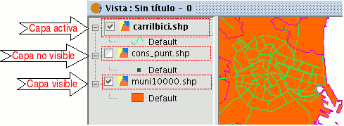
A check box next to each layer indicates whether it is "visible” or not.
Remember that an active layer is not the same as a "visible" layer. When a layer is “active” it is highlighted compared to the other layers included in the “Table of contents”. When a layer is activated, gvSIG is notified that the elements of this layer can be worked with.
The order of appearance of the layers in the “View” is important because it ties in with the display order. Layers made up of text elements, points and lines are placed at the top whilst the polygonal layers and images which make up the background of the view are placed at the bottom.
To move the layers in the ToC, place the cursor over them, left click on the mouse and drag the layer to the required position.
The layers in the ToC can also be selected by using the Control and CAPS keys.
Crear una agrupación en el ToC
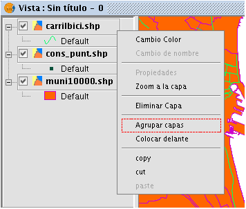
From version 0.4 onwards, gvSIG allows several layers to be grouped together. This is useful because it means a large number of layers can be kept in the ToC without taking up a lot of space. This option also allows operations to be carried out on all the layers that make up a group at the same time. To group a set of layers together, select the layers, click and hold down the CAPS key and right click on the mouse on any of the layers and select the “Group layers” option.
The following dialogue window appears and a name for the new grouping can be input.
When the name of the new grouping has been input, it appears in the ToC as shown below.
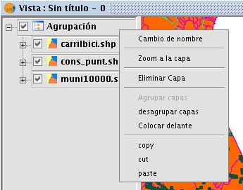
To undo a grouping, right click on the grouping so that the contextual menu appears. Select the "Ungroup layers" option.
Navegar/Explorar la vista
Navegar/explorar la vista
There are several tools you can use to navigate around the map. These are basically zooms and panning.
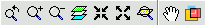
Zooms y desplazamientos
You can activate these tools by clicking on the "View” menu and then on “Navigation".
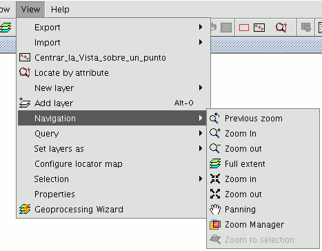
or by using the button bar which is quicker. Zoom in: Enlarges a particular area of the view.

Zoom out: Reduces a particular area of the view.

Previous zoom: Goes back to the previous zoom used.

Full extent: Full zoom of the total area included in all the layers of the view.

Panning: This allows you to change the view zoom by dragging the viewing field all over the view with the mouse. Click and hold down the left button of the mouse then move the mouse in the direction you require.

Zoom to selection: Full zoom of the total area of all the selected elements.

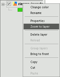
Zoom to layer: To zoom to the layer, right click on the selected layer in the ToC, or click on the “Zoom to layer” option in the contextual menu.
Gestión de encuadres
You can access the “Zoom manager” from the tool bar by clicking on the following button:

or from the “View” menu, then “Navigation” and “Zoom manager”.
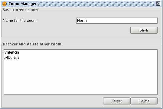
By clicking on the “Zoom manager” you can save a zoom so that you can go back to it at a later stage.
This tool can be used to name the current zoom of the view with the text bar which appears in the window.
Click on “Save” and the zoom currently in the view will automatically be added to the “Zoom manager” text box.
You can create and save as many zooms as you wish. Use the "Select” and “Delete” buttons to manage your working areas.
Configurar localizador
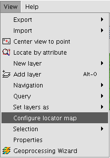
The locator is a general map which is displayed in the bottom left hand corner of the view's window. It is used to show the working area (main window zoom). Click on “View” in the menu bar and select “Configure locator map”.
A window appears in which we can add layers (we can add the same types of layers as in the view) which will make up part of the locator map. This window can also be used to remove layers or edit the layers’ legends.
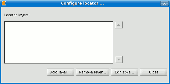
When you click on the “Add layer” button, the following window appears
This new function allows the layer loaded in the locator map to be reprojected. To do this, click on the button next to “Current projection when you have selected the layer you wish to load in the locator map.

In the following window, select the reference system you wish the layer to have in the locator map and click on “Finish” for the changes to take effect.
Herramientas de consulta
Herramienta de información
You can access the information tool via the following button in the tool bar

or by going to the “View” menu bar, to “Query” and then to “Information”.
The “Information Tool” is used to obtain information about the map elements.
When you click on an element using this tool, gvSIG shows the selected element’s attributes in a dialogue window. However, the layer of the element you wish to identify must previously be activated.
Medir áreas
You can access this tool via the following button

or by going to the “View” menu and then to “Query” and “Measure area”.
This tool works in much the same way as “Measure distances”. Click on the point that represents the first polygon vertex that defines the area to be measured. Move the mouse and click on each new vertex until you reach the last one, then double click so that the application knows there are no more.
The calculation for the measured area appears at the bottom right of the view window.

Medir Distancias

This tool provides information about the distance between two points. You can also access the tool by going to the “View” menu, to “Query” and then to “Measure distances”.

Firstly, make sure you have correctly defined the units of measurement (metres by default).
Remember that the units can be defined in the “Project manager” in the view properties or from the “View” menu and the “Properties” when working in a view.
You can use the measure distance tool by clicking on the mouse at the source point and dragging it to the destination point.
You can take as many measurements as you like. Double click on the last one to finish.
The calculation for the measured distance appears at the bottom of the view window. Both the distance of the last measured segment and the total distance are shown.
Selección de elementos
Introducción
You can select one or several elements or items by making either a graphic request or an alphanumeric request.
The selected data are shown in the view in the colour you have configured (by default this is yellow).
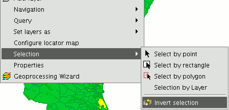
You can access the different ways of selecting elements by going to the tool bar or by going to the “View” menu and then to “Selection” as long as the layer you wish to work with has already been activated in the ToC.
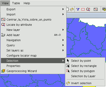
Selección por punto

This is the basic selection method and consists of clicking on the element you wish to select.
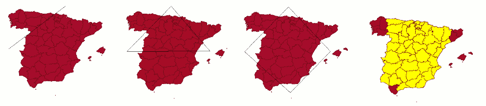
Selección por rectángulo

This allows you to select the elements which are partly or wholly located inside a rectangle.
To define the rectangle, place the cursor point over the position you wish to start to draw the rectangle in, left click on the mouse and hold the button down until you have defined the area you wish to select.
Selección por polígono

This allows you to select elements which are partly or wholly located inside a polygon.
To define this polygon, place the cursor in the part of the view you wish to draw the selection polygon in. Left click on the mouse in the view to add the polygon vertices.
When you have finished, double click on the mouse. All the elements which are located inside the polygon or which intersect with any of its sides will be selected.
Selección por capa
You can access this tool by going to the “View” menu then to “Selection” and “Selection by layer”. It allows you to select elements in the active layer based on the selection made in another layer.
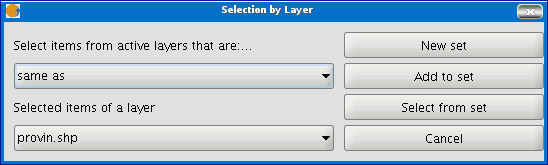
The options available using this tool are:
- 1.New set: This creates a new selection set.
- 2.Add to set: This creates a selection set based on the previous request and the current request.
- 3.Select from set: This creates a selection set from what has already been selected, the current selection request is extracted from the previous one.
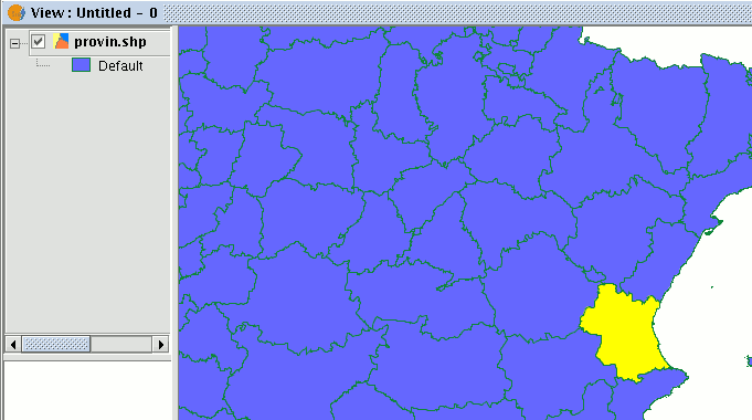
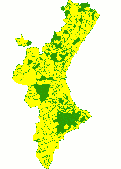
An example of how to use this tool consists of selecting the cities and towns of the Valencian Region whose municipal boundaries are affected by flood risks.
We start with a shape file with the areas of the provinces in the Valencian Region which are subject to flood risks.
Then the layer corresponding to all the cities and towns in the Valencian Region is added. Pre-select the full flood risk layer.
We go to the “Selection by layer” tool. Use the “Intersect with” option in the first pull-down menu, “Select items from active layers that are:…”.
Use the “riesgo_inundación_25000_completo” option in the second pull-down menu “Selected items of a layer”.
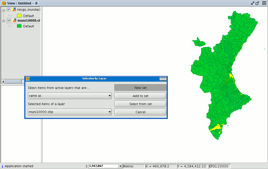
We can now click on “New set” and the layer with the new selection will appear.
Selección por atributos
You can access this tool using the following button:

gvSIG allows selections to be made using requests (filters). Selecting elements by attributes allows you to define exactly what you want to select, including several attributes, operators and calculations.
Requests can be made using logical operators, such as “equals” “more than” “different from”, etc.
If you press the “Filter” button in the tool bar, a dialogue window will appear to define your request.
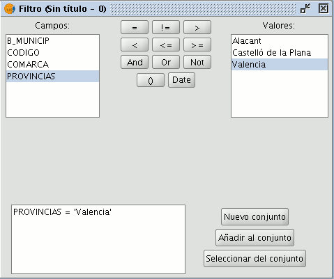
1.Fields: Double click on the field you wish to add to your request from the “Fields” list in the layer.
2.Logical operators: These allow you to insert a logical expression into your request by clicking on them.
3.Values: This shows a list with the different values the selected field has. If you wish to add a value to the request, double click on it.
4.Request: This is the window which represents the request to be made. You can write here directly.
5.Selection buttons: These buttons make the request using:
New set (deletes any previous selections).
Add to set (adds the elements selected by the request to the existing elements).
Select from set (makes the request from the selected elements).
Invertir selección
When you have made your selection, you can click on the following button in the tool bar

or you can go to the “View” menu then to “Select” and “Invert selection”
and invert the previous selection as shown below.
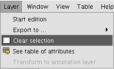
Borrar selección

If you click on this button, the selected element set will once again become empty. You can also access this option by going to the “Layer” menu then to “Clear selection”.
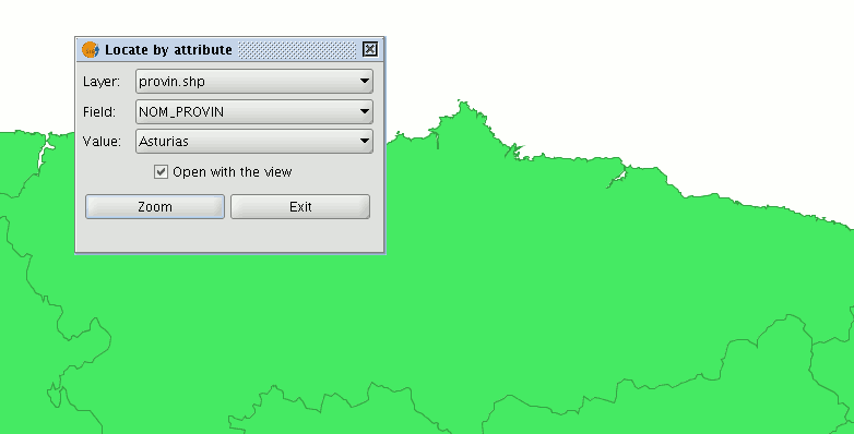
Localizador por atributo
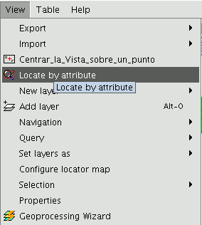
This tool allows you to zoom in on areas of a layer by specifying the value of a particular attribute. You can access this tool by clicking on the button

or by going to the “View” menu then to “Locate by attribute”.
When the tool is selected, the following window appears
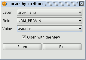
You will find all the layers loaded in the ToC in the “Layer” pull down menu. The fields associated with the chosen layer are included in the “Field” pull down menu.
The data included in the selected field appears in the "Value" pull down menu.
If you mark the “Open with the view” check box and decide to close the view, the “Locate by attribute” window will appear the next time you open the view.
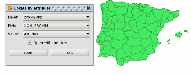
When you have made the selection, click on the "Zoom" button and the chosen area will be shown in the view.
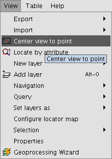
Centrar la vista sobre un punto
This tool allows you to locate a point in the view by its coordinates and to centre the view on this point.

You can also access the tool by going to the “View” menu then to “Centre view on a point”.
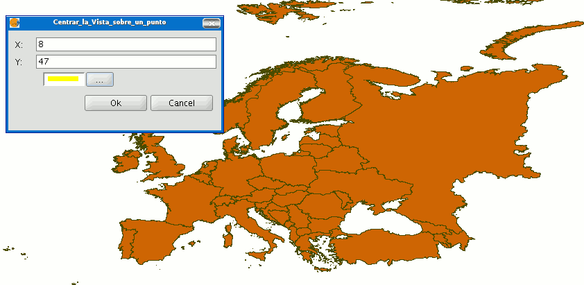
When you have accessed the tool, a dialogue box will appear in which you can input the required coordinates and select the point colour.
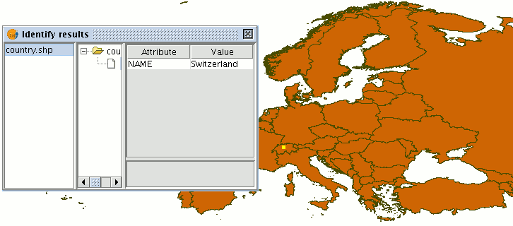
When you click on the "Ok" button, the view centres on this point and the information window that corresponds to this point appears.
Catálogo. Búsqueda de geodatos
Introducción
The catalogue service allows you to search for geographic information on the Internet. gvSIG offers a user-friendly interface which allows you to find geodata and load it in the view, as long as the nature of the data allows this.
Conexión con un servidor
Before you can carry out a search, you will need to connect to a catalogue server. To access the wizard, you will first need to open a view and then click on the following button:

The first window of the catalogue opens. Input the required parameters to connect to a server. These include:
- The server address.
- The server protocol, which in the case of the catalogue can be:
- Z39.50: General information retrieval protocol.
- SRU/SRW: Variant of Z39.50.
- CSW: Catalogue protocol defined by the OGC in the “Catalogue Interface 2.0” specification.
- Data base name: You only need to indicate the data base you wish to connect to in the case of z39.50. If no value is input you will connect to the default data base.
Then click on the “Connect” button. If the connection is made and the server supports the specified protocol, a new window will appear to start the search.
Búsqueda
To carry out a search, you need to fill in the fields that appear in the following form.
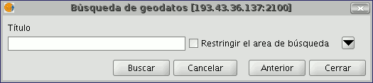
Click on the button and the window will drop down to show more fields which will allow you to carry out an advanced search. The fields you can search in are set by the server. This means that some of the search fields in this form may have no effect in some servers.
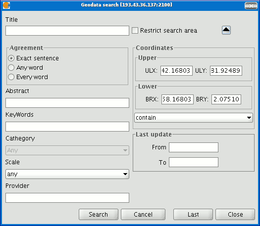
If you change the view zoom, the new coordinates will be reflected in this form. If you wish to restrict the search area enable the corresponding check box. Then click on “Search” and wait for the search to be carried out.
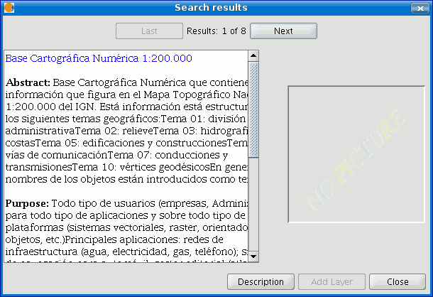
Visualización de los resultados
If the search has been successful, a new window containing the search results will open.
Use the “Previous” and “Next” buttons to see each of the results obtained.

The left-hand side of the window shows information about the metadata obtained. If you wish to see all the information, click on the "Description" button.
You will also be able to see a miniature image at all times, metadata permitting.
If the metadata has any geodata associated to it, the “Add layer” button will be enabled.
gvSIG can currently recognise different types of associated resources, such as WMS, WCS, Postgis tables and web pages.
If you click on this button, a new window will be opened and will show all the resources the application has been able to find.
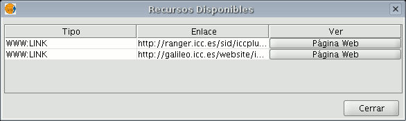
If you click on a WMS, WCS or Postgis type resource, the new layer will automatically be loaded in gvSIG. If the resource is a web page, for example, the operating system’s default browser.
Nomenclátor
Introducción
A gazetteer is a data set in which a link is established between a toponym and its geographic coordinates.
gvSIG has a catalogue client which allows you to search by toponyms and centre the view on a specific point.
Conexión con un servidor
Create a view first and open it. The following button will appear automatically in the gvSIG tool bar.

Click on the button. A wizard opens to help you to carry out a search. The parameters to be input are:
- The server address.
- The server protocol, which in the case of the gazetteer can be:
- WFS-G: Toponym search protocol defined by the OGC.
- WFS: Although this protocol was created with a different purpose in mind, it can be used for a toponym search, as long as it has a text attribute in one of the tables. This protocol also allows you to carry out a “Feature” search in any other field, but not necessarily a text attribute.
- ADL: Protocol specified by the Alexandria Digital Library.
- IDEC/SOAP: Protocol that uses the Catalonian Cartographic Institute (ICC) gazetteer web service.
When you have input all the parameters, click on the "Connect" button and wait until the server is found and accepts the specified protocol. If it is accepted, a new window will appear to start the search. If not, an error message will appear.
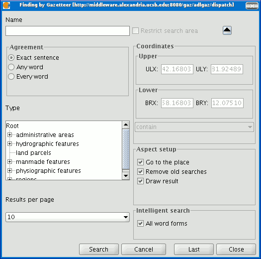
Búsqueda
To carry out a search, you will need to fill in the criteria that appear in the following form. You can see the simplified form or carry out an advanced search by clicking on the button in the top right hand corner. This drops down the window.
If you change the view zoom, the new coordinates will be reflected in this form. If you wish to restrict the search area activate the corresponding check box. There are also three options in the “Aspect set up” box which you can use to set up the search view:
Zoom to search: This puts the toponym found in the centre of the gvSIG view.
Delete old searches: This deletes all the texts found in the previous searches from the view.
Draw result: This draws a point and a text label in the place the resulting toponym has been found.
When you have filled in all the fields in the form, click on “Search” and wait for the search to be carried out.
Visualización de los resultados
A new window containing the search results will open. Use the “Previous” and “Next” buttons to move through the different pages of results.
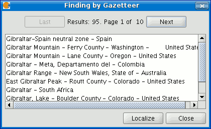
Finally, select the toponym required and click on “Localise”. The gvSIG view will centre on the point the toponym is located in.
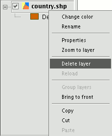
Eliminar capas
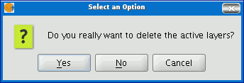
To permanently remove the active layers from the view, right click on the layer in the ToC and select the “Delete layer” option.
A confirmation dialogue appears.
Exportar capa
Introducción
The “Export to...” tool allows you to save the elements selected in a layer in a different format. If no elements have been selected the whole layer will be exported. At the time of going to press the export formats supported by gvSIG were shape, dxf, and postgis and gml.
Exportar a shape
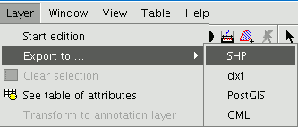
Select the “Layer” option from the menu bar then go to “Export to…/shp”.
If you have selected elements in the layer to be exported, gvSIG will tell you how many elements are going to be exported and will ask for confirmation before carrying out the operation.
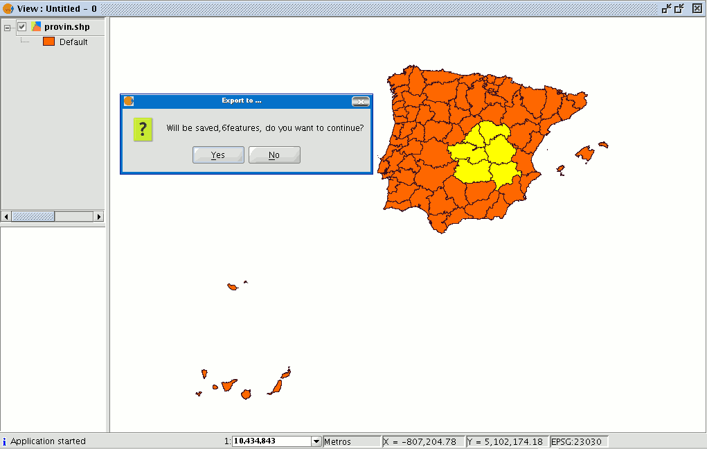
If you continue with the operation, a dialogue box will appear in which you will be asked to select the file the new shape is to be saved in.
When you have accepted, a new message will appear asking whether you wish to insert the new layer into the view.
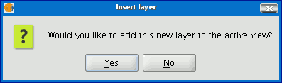
If you click on “Yes”, the layer will be added to the active view.
Exportar a dxf
Select the “Layer” option from the menu bar then go to “Export to…/dxf”.
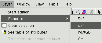
Follow the same process used for exporting to shape.
Exportar a postgis y Oracle
Select the “Layer” option from the menu bar then go to “Export to…/postgis”.
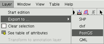
If you have selected any elements, a window will appear telling you how many elements are going to be exported (as in exporting to shp and dxf).
If you have selected any elements, a window will appear telling you how many elements are going to be exported (as in exporting to shp and dxf).
Remember that if the table already exists in the data base, the information it contains will be deleted.
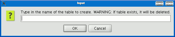
Write the name of the table and click on “Ok”. A new window appears in which you will have to input the parameters of the data base connection.
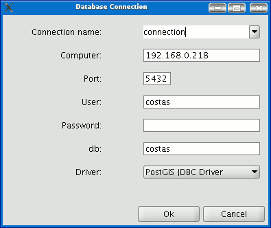
he parameters are:
Name: Name of the connection.
Computer: IP address of the computer the data base is hosted in
Port: Port on which the computer is listening to the postgreSQL service.
**User:**User name recognised by the administrator to make the connection
Password: User password required to validate the connection. db: The data base the new table is to be created in.
Driver: Driver required for the data base. (At the time of going to press, drivers for postGIS and mySQL were available). When you have input the connection parameters, click on “Ok”.
Exportar a gml
Select the “Layer” option from the menu bar then go to “Export to…/gml”.
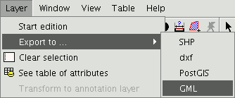
Follow the same process used for exporting to shp or dxf.
Exportar a raster
This tool allows you to extract portions of a raster layer using a selection in the view or by inputting the coordinates that define the portion to be extracted.
It allows the user to change the spatial resolution of the clipping or of the whole image, choose the bands to be extracted or generate a new raster layer for each of the original bands.
To access this option, go to the ToC and select the raster layer you wish to select a portion of.
Then go to the Layer/Export to menu and select the “Raster” option.
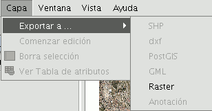
The following window appears:
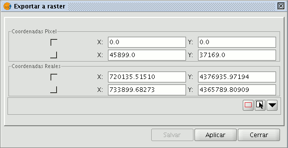
Image clipping
There are two ways of selecting an area to be clipped from the original raster layer:
You can use the text boxes in the window to input the data which correspond to:
- Real coordinates: If the source image is georeferenced.
- Pixel coordinates: If the source image is not georeferenced.
You can also make your selection directly from the view by clipping the whole image or selecting a part of it.
This button allows you to obtain a clipping from the whole image.
This button allows you to obtain a clipping from a selected area in the view. Place the cursor over the image, then click and drag. Check that the text boxes are automatically completed.
If you wish to save the raster layer clipping you have created, click on “Save” and select the location you wish to save this file in. The image will be saved in TIF format.

Changing spatial resolution
The controls that allow you to specify the clipping’s (or whole image) spatial resolution are located in the Clip table, with the additional options panel pulled down (to pull this panel down click on the button). You can define the resolution by specifying the Cell size or the Width and Height of the raster layer to be generated in pixels as well as choosing the interpolation method using the resolution change. At the moment, only the “Nearest neighbour” option is operational.

Band selection
The original raster layer’s band list appears at the bottom of the Clip table. You can use this list to choose the bands the output raster layer will have if you enable or disable the check boxes in the Bands column. If you check the Create one layer per band option, a new layer will be generated for each of the bands checked in the list. The new layers will be added to the ToC.
Saving and Adding a raster layer clipping to the current view.
When you have established all the parameters which define the raster layer clipping you have made, click on “Save”. This opens a dialogue box which allows you to search for a directory to save the clipping in. If you wish to add the layer to the view, go to the “Add layer” button in the tool bar once you have saved the clipping.
Example of a raster layer clipping
This example shows how a clipping is taken from an orthophoto.
First, select the area by defining a rectangle in the gvSIG view.
When you have finished, the coordinates will automatically be input into the text boxes based on the selection. You can fine tune these selected values from the view by inputting the new value directly into the text boxes containing the data.
Then pull down the box. As the resulting image is to be resampled, not as much resolution is required. Therefore, go to the “Spatial resolution” section and select “Width x Height”. This enables the text boxes so that you can input the output raster layer resolution.
When one value is input the other one is automatically completed when you press Enter or when you exit the field, as the proportions between the width and height must be maintained.
The cell size for the chosen output resolution is also calculated. If “Cell size” had been chosen, you would have had to specify the size in metres for each pixel and thus the width and height for the chosen cell size would have been calculated.
You now need to select the bands you want the output layer to have. In this case, select them all as this is a three-band orthophoto and we want to include them all.
Finally, for our example, the “Create a layer per band” option needs to be enabled to do just this.
Each new layer will have the same data type as the original image. If you click on “Save” a dialogue box opens to indicate the directory and image name.
To retrieve the layers you have created, go to the Add layer” button and then to the directory they were saved in.
Exportar a imagen y WMC
Exportar a imagen
This option allows you to convert the active view into an image or raster file.
Select the “View” menu then go to “Export/Image”.
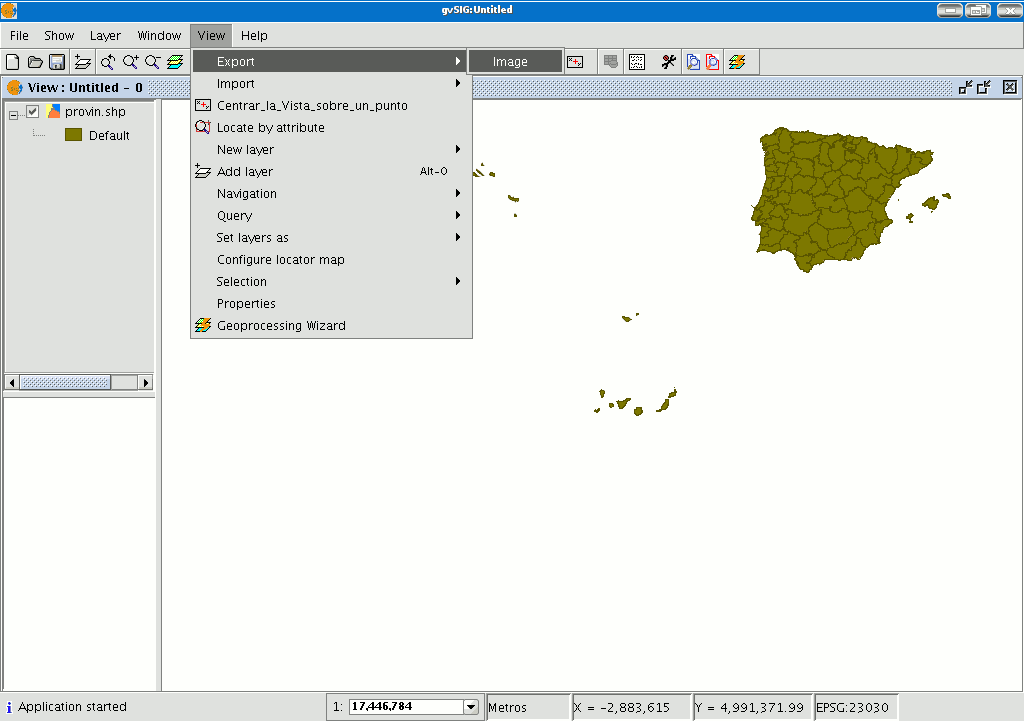
When you have selected the tool, a new window appears which you can use to edit the name of the image to be saved and the type of file (jpg, png...) you wish to save it in.
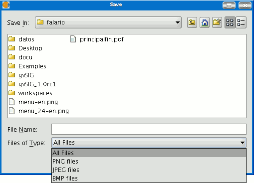
When you have saved the image, you can recover it from gvSIG by going to the “Add layer” tool and searching for a “gvSIG Image Driver” file type.
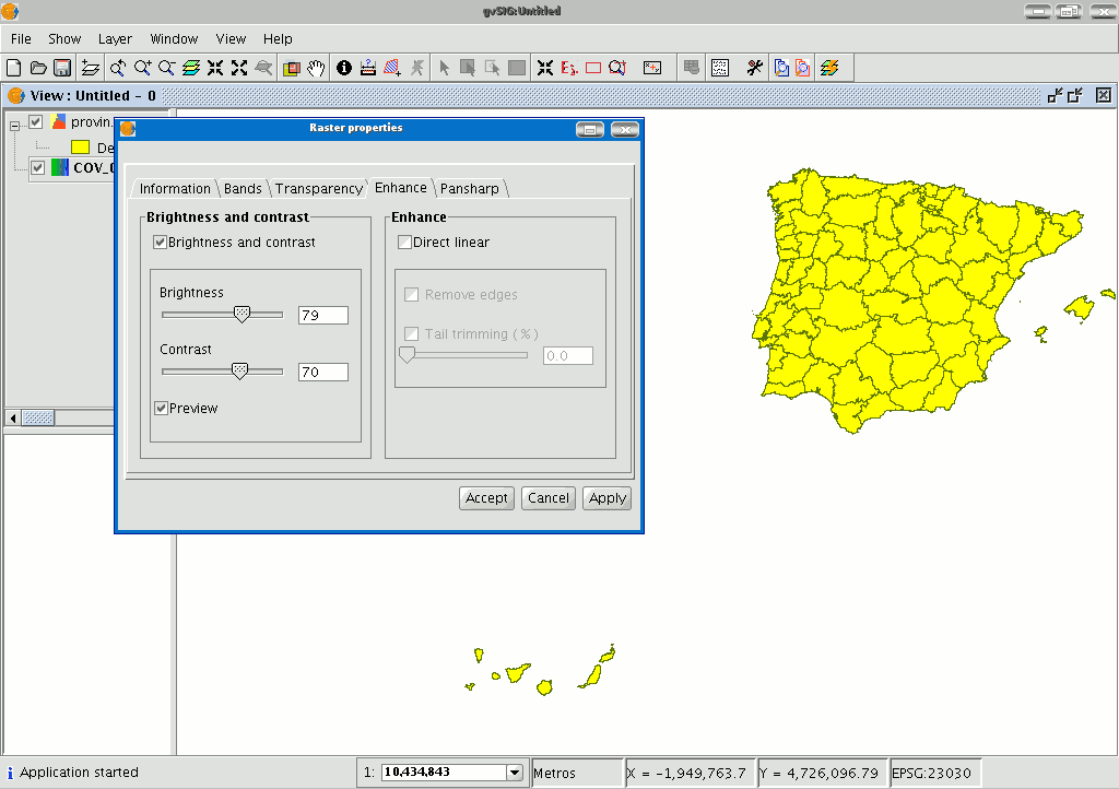
Use the ToC to check that the exported image is a raster layer by accessing its properties (right click on the layer in the ToC and then go to “Raster properties”).
Web Map Context
Introducción
Web Map Context (WMC) is another OGC standard (http://www.opengeospatial.org) which can be added to the list of standards of this type supported by gvSIG.
It can reproduce a view made up of Web Map Services (WMS) layers on any GIS platform which supports WMC. If your project has a view which contains WMS layers, you can export these layers. The result is an XML file with a specific format and .cml extension which can be imported by another platform on which the view it describes can be reproduced.
Exportar una vista a WMC
Web Map Context (WMC) is another OGC standard (http://www.opengeospatial.org) which can be added to the list of standards of this type supported by gvSIG.
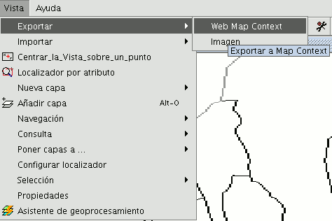
It can reproduce a view made up of Web Map Services (WMS) layers on any GIS platform which supports WMC.
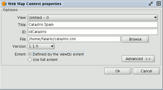
If your project has a view which contains WMS layers, you can export these layers. The result is an XML file with a specific format and .cml extension which can be imported by another platform on which the view it describes can be reproduced.
Exporting a view to WMC
Exports to WMC are currently limited to WMS type layers, although it is hoped that its functions will extend to all layers that comply with OGC standards in the future.
To obtain a WMC file, open a view in gvSIG and add the WMS layers you require.
Then go to the “View” menu and select “Export” and then “Web Map Context”.
The following dialogue will be shown.
N.B.: If you cannot find the "Web Map Context" option in the "Export" option, your project does not contain any WMS layers.
Basic mode only shows the compulsory properties which cannot be taken for granted by the application.
View: This defines which view is going to be exported to the WMC. The view which is currently active is selected by default.
Title: This is the title of the view which will be shown when your .cml file is loaded at a later date. The current title of the view is used by default but this can be changed.
ID: This field is also compulsory and represents a file ID which must be unique.
File: You can search for the place you wish to save the .cml file in from the "Browse" button.
Version: Use this tool to specify the WMC version you wish to use.
The version 1.1.0 is selected by default as it is the most highly developed and the most recommended. However, several applications and geoportals are often limited to a specific version.
gvSIG currently supports Web Map Context in its versions 0.1.4, 1.0.0 and 1.1.0.
Extent: This defines the extension of the map to be exported.
Defined by the view’s extent. This option only exports what we can currently see in the view.
Use full extent. This extension is better to use the full WMS layers depending on how their respective servers define them.
If you click on the “Advanced” button, the advanced configuration dialogue will drop down. This allows you to define more properties to obtain a complete WMC.
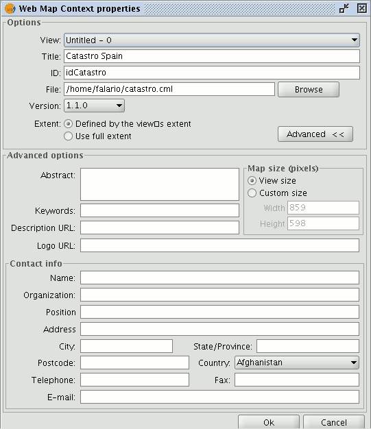
Abstract: This contains a summary of the view defined by WMC.
Keywords: This list of words allows you to classify and “metadata” the WMC.
URL description: If you have a web site which refers to this WMC, write its link here.
URL logo: If you have an image associated with this WMC, write its link here.
Map size (pixels): This defines the pixel size that the WMC-defined view will have. The current gvSIG view size is used by default but you can customise the size if you wish.
Contact info: Information that allows third parties to contact the WMC author.
Importar un WMC
Importing Web Map Context allows you to use gvSIG to open views with WMS layers which have been created with other platforms or with another gvSIG.
Use the "View” menu and select “Import” and then “Web Map Context”.
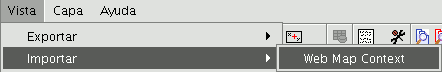
The WMC file selection dialogue opens.
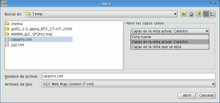
Choose the WMC file you wish to import. On the right, you can specify how you wish to view the layers.
New view: This adds a new view to the current project and loads the WMC as specified in the file.
Layers in the active (current) view: This option only appears if the active gvSIG window is a view. It allows you to quickly add the layers to the current view.
Layers in other view: This adds the layers defined by the WMC in the chosen view. In this option, a list of views appears to select the view that will contain the new layers.
Click on the “Open” button to import the file based on your preferences.
Capa de anotaciones
Introducción
This gvSIG tool makes advanced labelling easy.
The process creates a new layer which represents annotations.
The main features of this new layer can be summarised as follows:
- The new layer is only composed of the annotations created.
- The table associated with this new layer only contains the fields which refer to the text of the annotations (Text, Font, Colour, Height and Rotation).
- The layer created is always in .shp format, irrespective of the format of the original layer.
Crear una capa de anotaciones
To create an annotation layer, first select the layer from the ToC (Table of Contents).
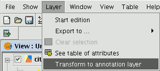
In the menu bar, select the “Layer” option, then select “Export to” and finally select the “Annotation” option.
This option opens the wizard which will guide you through the steps required to create the annotation layer.
In the wizard’s first window, select the data which gvSIG requires to carry out the operation from the pull-down tab:
Duplicate control: Select either “None” or “Centred” to choose the position in which you wish the annotations to be inserted.
Centred: A label is created for each value and this will be inserted in the centre of all the labels which are the same.
None: A label is inserted for each value, even if these are repeated.
Select the field to be labelled: Choose the field which contains the text you wish the labels to show.
If you do not wish to modify the format of the annotations created by gvSIG and prefer a standard format, click on “Finish”. If you wish to customise the format, click on “Next”.
The wizard’s second window allows you to select the fields of attributes of a a table (if there are any) which contain the values which allow you to customise the labelling.
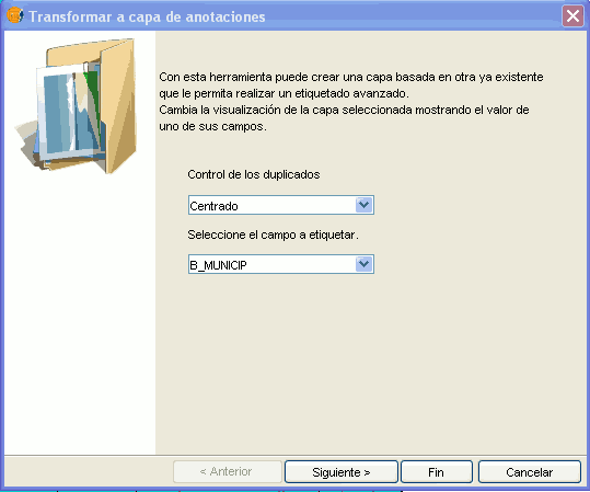
The following parameters can be customised.
Slope – the slope the annotation will have in the view.
Colour – annotation text colour.
Height – annotation text height.
Units – units in which the value assigned to the “Height” field are to be measured.
The options currently available are map units or pixels.
Font – annotation text font.
Set the values to be used for customising the required parameter (by pulling down the list).
Leave the default value in the fields you do not wish to customise.
Click on “Finish” when you have input these changes.
Edición de una capa de anotaciones
An annotation layer can be edited like any other layer. To start an editing session in gvSIG, select the layer in the Table of Contents and then select the option “Start edition”.
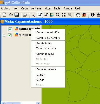
When you start an editing session, an option appears in the menu bar called “Modify annotation”. This will allow you to individually customise the annotation you wish to change.
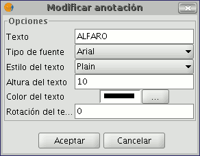
When you click on this button, the appearance of the cursor will change. You may graphically select the annotation by clicking on the point associated with the text and then access a set of properties shown in the following image.
Propiedades de la capa de anotaciones
If we select the “Properties” option from the annotation layer contextual menu, the following box appears:
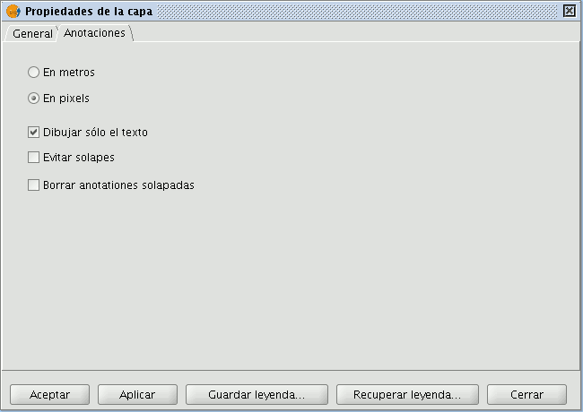
The “Layer properties” box has two tabs. The “General” tab allows you to access the general properties of the layer and the “Annotations” tab allows you to select: whether you wish the annotation text to be shown in pixels or metres in the view.
Whether you want only the text to appear (select the “Draw text only” option) or if you prefer the text to be accompanied by a location point (deselect the “Draw text only” option).
However, remember that this point is useful, for example, to move the annotation or to access the “Modify annotation” window.
If you wish to avoid overlays, activate the “Avoid overlays” option.
If you wish to eliminate overlaying annotations, activate the “Clear overlaying annotations” option.
Añadir la capa de anotaciones a la vista
To add an annotation layer, click on the “Add layer” button in the tool bar

and select the “Annotation” tab.
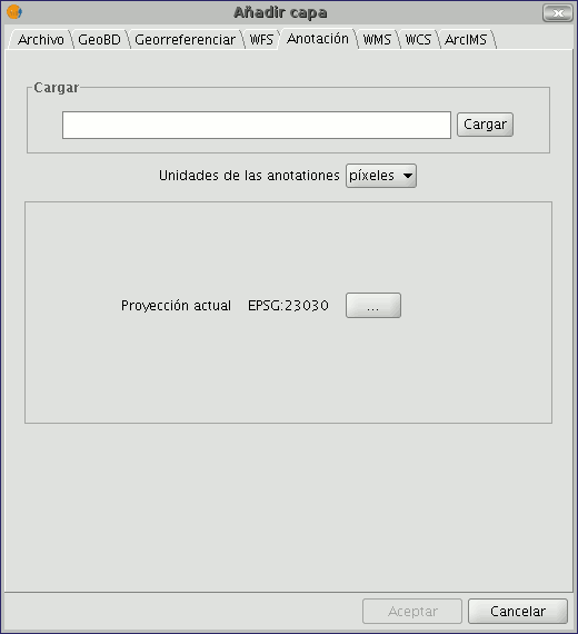
In the box you can select the annotation layer you wish to load, in addition to the units in which the annotations are displayed (pixels or metres) and the projection of the layer.
Ejemplo de creación de capa de anotaciones
The following image shows how an annotation layer is created out of a polygon layer called “muni10000.shp” which contains all the towns in the Valencian Region.
In the first window of the wizard, insert the type of duplicate control you wish to use and select the field which contains the text to be shown.
This is the field in a layer’s table of attributes which contains the name of the town.
If you do not wish to customise the presentation, click on “Finish” and indicate where you wish the new annotation layer to be saved.
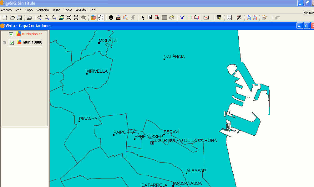
The following image shows the result (the rest of the fields in the wizard are left with their default values and this one is zoomed in) of creating the “annotation layer”.
The annotation layer which has been created is the one in red called “Towns” in the Table of Contents.
Tratamiento de imágenes ráster
Salvar a ráster
First of all, load the cartography you need to make a clipping onto a gvSIG view. Select the “Save as raster” tool which appears in the tool bar.

Now select two points in the view to define the rectangle that will contain the area to be saved. The following dialogue box then appears. If the rectangle you have marked is too small, this box will not appear and you will have to select a larger rectangle.
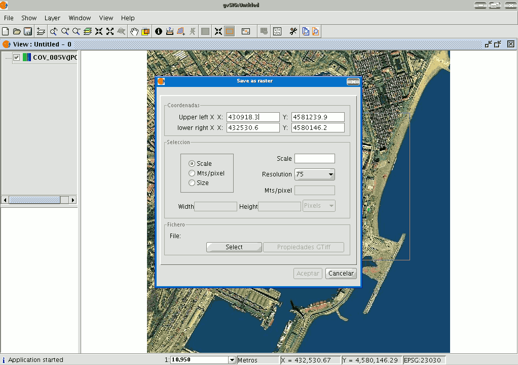
The coordinates of the points which delimit the selected area in the view appear at the top of the “Save as raster” dialogue. These coordinates can be changed manually.
The “Selection” area appears in the centre of the dialogue.
This includes three selection methods:
Scale. If you select “Scale”, the “Scale” text box and the “Resolution” pull-down menu are enabled. The pull-down menu values correspond to the points per inch in the exported image.
Input a value for the scale and press “Enter”. The Mts/pixel values and the “Width” and “Height” size of the output image are recalculated.
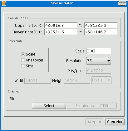
Mts/pixel: If you select “Mts/pixel” from the three radio-buttons column, the text box to input this value will be enabled. Input a Mts/pixel value and press “Enter”. The “Scale” value and the size (“Width” and “Height”) of the output image will automatically be recalculated.
Size: If you select “Size”, the text box to input the “Width” and “Height” values will be enabled. When you input one of these values, the other will be recalculated automatically to maintain the height/width proportions.
The remaining data (“Mts/pixel” and “Scale”) will also be recalculated automatically. You can also select the unit of measurement you wish to see the values in via the “Pixels” pull down menu.
Click on the “Select” button to choose where you wish to save the image.
The most suitable driver will be loaded according to the type of file you choose (N.B. watch how the button to the right of “Select” changes), i.e. when a .jp2 output file is selected for example, you can open the properties box which corresponds to a Jpeg2000 format.
The formats available to save a file are geoTiff, jpg (georreferenced with a worldFile) and jpeg2000.
An ecw extension can be selected exceptionally and only with Linux kernel 2.4.
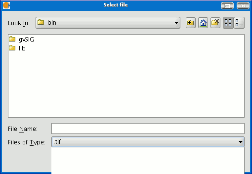
When you select the output file the properties button is enabled.
For geoTiff files, a box similar to the one below appears:
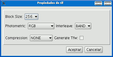
Block size: The block size defines the amount of data read each time so it can be compressed. The greater the block size the faster the compression speed but more memory is used.
Photometric: [MINISBLACK | MINISWHITE | RGB | CMYK | YCBCR | CIELAB | ICCLAB | ITULAB].
This assigns the photometric interpretation.
This is RGB by default, because the input image has 3 byte-type bands. Interleaving: [BAND | PIXEL]. The tiff files have band interleaving. Some applications only support pixel level interleaving. In these cases, this option can be modified. Compression: [LZW | PACKBITS | DEFLATE | NONE] This assigns the compression to be used. The default option is none.
A table like this will be obtained for jpg.
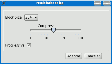
Block size: The block size defines the amount of data read each time so it can be compressed. The greater the block size the faster the compression speed but more memory is used.
Compression: This allows the image’s compression level to be adjusted.
Progressive: This allows you to make progressive jpgs.
When the image has been selected and the properties have been adjusted, click on “Ok”. A progress bar appears.
This process may take an extremely long time depending on the size of the output image.
It can take from a few seconds to several days. Thus, it is advisable to control the size of the output image via the number of pixels so we are not taken by surprise.
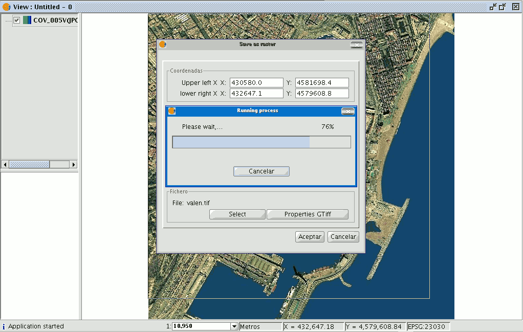
When the process finishes, a statistics table indicates the saved image path, the disk size of the output image, the length of the process and whether the image has been compressed or not.
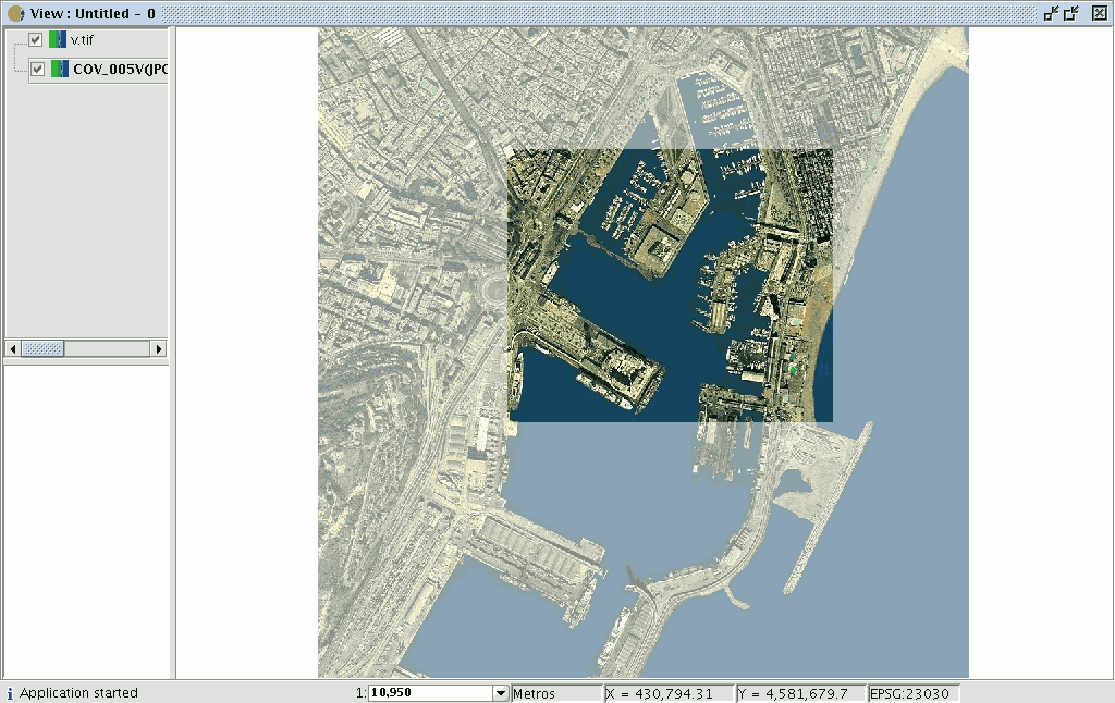
To check that the georeferencing has been correctly carried out, you can load the image you have saved as another layer and apply a transparency.
Georeferenciación con cartografía base y puntos de control
Introducción
The gvSIG programme allows an image to be georeferenced (.jpg, .tif, .gif, .png) using control points on a georeferenced base map. Firstly, the georeferenced base map needs to be loaded (in raster or vector format or both) to a gvSIG view.
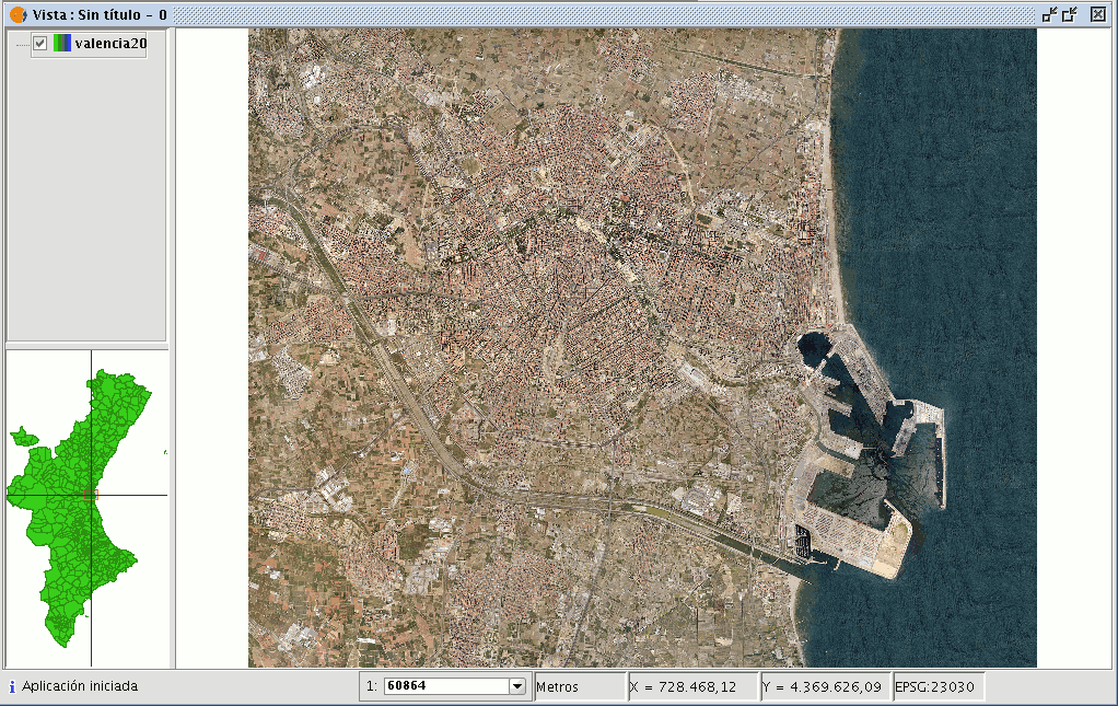
Secondly, the image to be georeferenced must be added. You can load this image by going to the “Add layer” tool and selecting the “Georeference” tab. Use the “Load” button to access the image you wish to georeference.
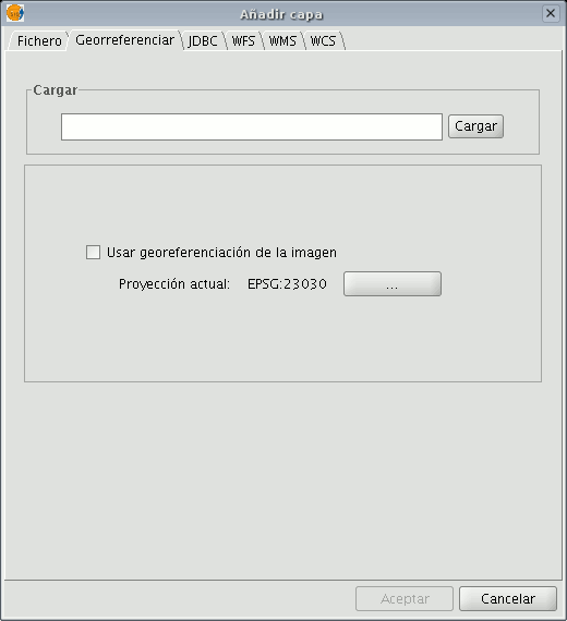
If you enable the “Use image georeferencing” check box and the image is georeferenced, it will be added to the view with its current georeference. If it is not, the image will be loaded in the centre of the view. You will then find a browser button which can be used to select the map projection.

When you have finished the process, click on “Ok”. The image to be georeferenced will appear in the view and will have an asterisk “*” in the ToC to indicate that this is the layer the process is being carried out on. A new window will also appear to carry out the georeference process but first, the image to be georeferenced will have to be moved closer to the base map’s reference zone so that you can select the control points more quickly.
Aproximación de la imagen a georeferenciar
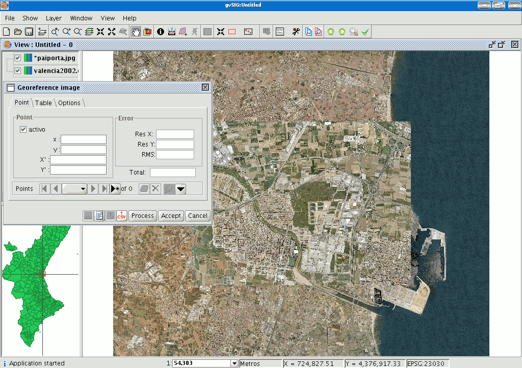
If the layer to be georeferenced is selected in the ToC, four new buttons will appear in the tool bar.
This button resizes the image to be georeferenced.

The image size can be modified and brought closer to the base map scale.

Select this tool and go to the image to be georeferenced.
A frame will be created around the image. If you place the cursor on one of the image sides, it will turn into a double arrow. This will then allow you to modify the frame size by moving the cursor.
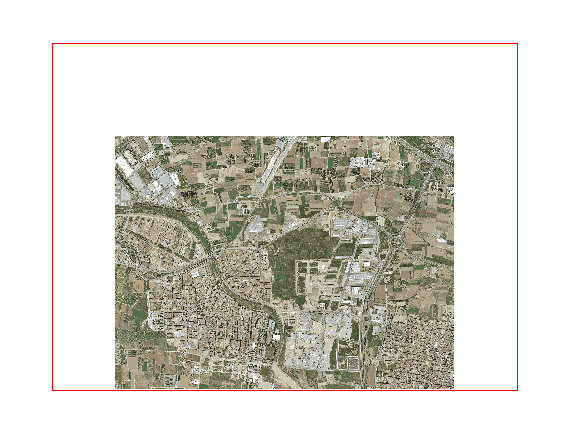
The newly created frame boundaries will become the new reference size for the image being georeferenced.

This tool allows you to move the image to be georeferenced around the view and thus bring it closer to the reference base map.

This tool takes you back to the previous position of the image to be georeferenced in the view.

This tool is activated when the previous tool has been used and allows you to redo what you have previously undone.
Selección de puntos de control
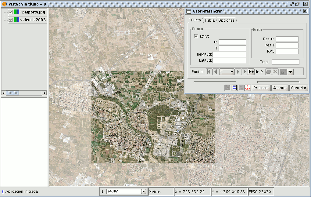
Click on the “New point” button in the “Georeference” dialogue and go to the view.

Place the mouse pointer over the image to be georeferenced and look for a control point. This point is defined as a red circle with a cross in the middle. If you move outside the boundaries of this image, gvSIG shows an error message and you will have to select a point once again. If you click on the following button

two small windows will drop down. In the left-hand window, the location of the created control point appears over an image zoom, as the following image shows.
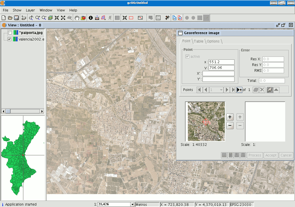
If you wish to specify the point further, you can zoom into the image using the zoom tools in the centre of the dialogue box.

If you then click on the point in the mini view and drag it you can move its location.
These changes will automatically be reflected in the gvSIG view.
When you have marked the control point on the image to be georeferenced, this will disappear from the view (this option is marked by default in the "Options" tab in the "Georeference" window and can be modified at any time) and will only leave the base map with the destination point marked on the view.
In this case, the point is defined by a blue square with a cross in the centre.
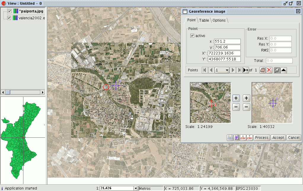
You can do the same with the mini view on the right as you did with the left, i.e. if you wish to move closer to the point location, you can zoom into the right-hand image and drag the point over the view to place it more precisely.
You can also specify the points in the text boxes in the georeference dialogue window. When the points have been input, press “Enter” and the point will be located in the view.
Remember that the “X” and “Y” text boxes belong to the image to be georeferenced and that “Longitude” and “Latitude” correspond to the georeferenced image. If you have made a mistake with the point and wish to delete it, click on “Remove selected point”.

If you click on this button, a confirmation message will appear.
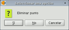
If you click on "Yes", the point will be deleted. If you wish to remove all the points, click on the “Remove all the points” button.

The control point selection must be repeated as a minimum of three points are required for georeferencing, although at least nine are advisable.
There is another series of tools in the “Georeference” window:

This tool allows you to go to the first control point, to the previous point, search for control points using a pull-down menu, go to the following control point and go to the last pull-down point respectively.
This button allows you to select control points from the view. Firstly, select the control point of the image to be georeferenced and finally, the control point of the destination coordinate.

You can disable an input control point via the "Active” check box in the “Point” tab. This means that the point will not be used in the error and georeference calculations and the symbols will not appear in the view. If you need the point again, you can enable the check box.
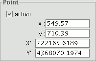
If you click on the “Table” tab, a table will appear with all the points and their errors. This table can be enlarged to show more information.
Guardar y cargar puntos de control
When you have finished the georeference process, you can save your control points by using the following tools:

In a metadata file associated with the image with the .rmf extension (if data already exists in this file, gvSIG will warn you that it is going to overwrite it).

In a .csv file: In this case, a dialogue window opens to select a file to save the data (X, Y coordinates and the errors in X, Y and RMS).

However, if you wish to add points from a file, use the following tools to retrieve .rmf control points associated with the image.

To load control points from a .csv file.
N.B.: You can also save the georeference points in the table panel.
Opciones
You can use the “Options” tab in the georeference window to enable and disable some of the options according to your preferences.
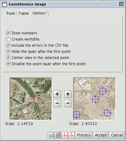
Restricciones
It is currently only possible to georeference bmp, gif, jpg, png and tif formats.
Brillo y Contraste y Realce
Applying “Brightness and Contrast” and “Enhance” filters to raster images. Firstly, load the cartography in raster format in a view and right click on the name of the raster layer selected in the ToC.
When the menu appears select the “Raster properties” option.
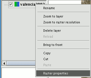
Then go the “Enhance” tab.
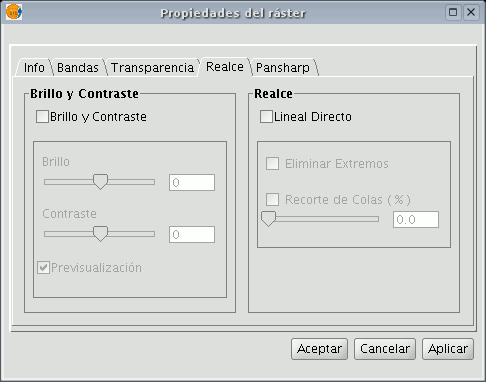
You will see that the “Brightness and contrast” and “Enhance” adjustment panels are disabled by default. These panels can be enabled by checking the boxes at the top of each panel.
If these check boxes are disabled no filters will be applied to the image even though the values have been input into the panel.
If, at any time, any of these filters have been applied to the image, the values will appear in the panel.
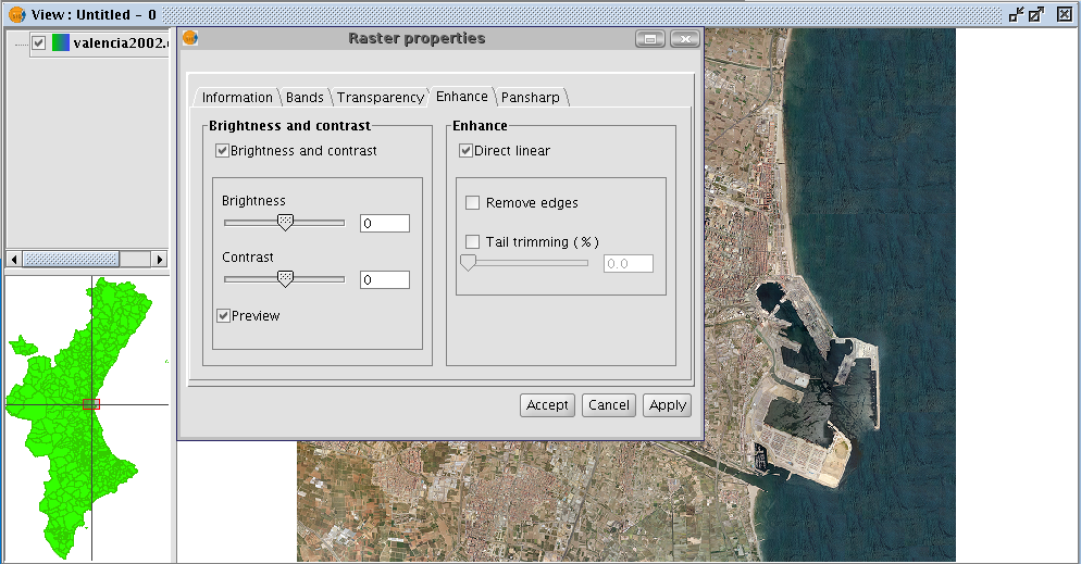
You will find two slider controls in the “Brightness and contrast” panel.
Values can be modified by using the slider or by directly inputting the values in the numerical field on the right and pressing “Enter”.
The brightness and contrast increase range goes from -255 to 255. To fine tune these values without having to input them in the numerical field, click one end of the slider control to either increase or decrease the value, unit by unit.
You will find a “Preview” check box in the panel. This is useful for obtaining a preview of the image without having to “Accept” or “Apply” changes every time they are made. If this check box is enabled, the image is refreshed with the new filters when the mouse button is released after modifying the brightness or contrast values using the slider control or when “Enter” is pressed if the numerical field has been used to modify the value.
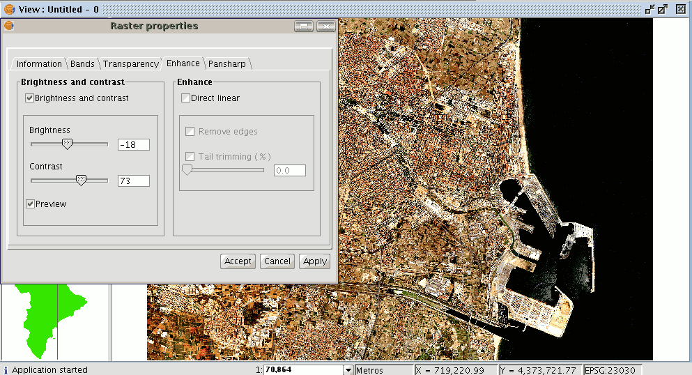
When brightness and contrast filters are applied the previous image takes on the above appearance.
When “Cancel” is pressed, no changes are applied and the input values are lost.
If you press “Accept” and you return to “Raster properties” you will see that the previously input values have been saved.
Transparencia por píxel
This assigns transparency to a raster based on the colour of its pixels. To assign this transparency, first load the cartography, then place the mouse pointer in the ToC over the raster layer you wish to modify. Right click and the contextual menu will appear.
Select the "Raster properties" option. When the dialogue box opens, select the "Transparency" tab. Only the top part of the panel corresponds to this tool. Enable the “Activate” check box and the controls that correspond to this function will be activated.
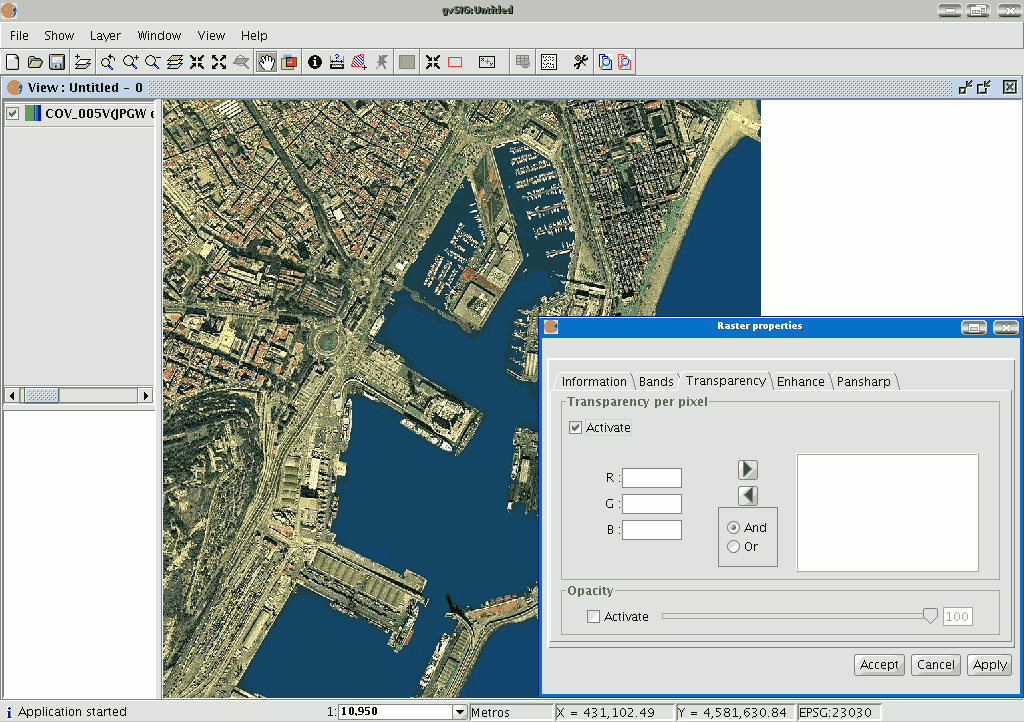
You can write the required combination of red, green and blue values in the “R”, “G” and “B” text boxes. When you have input these values, you can add them to the list with the right-facing arrow. These values will be added with an AND (&) if the “And” check box is enabled and with an OR (|) if the “Or” check box is selected.
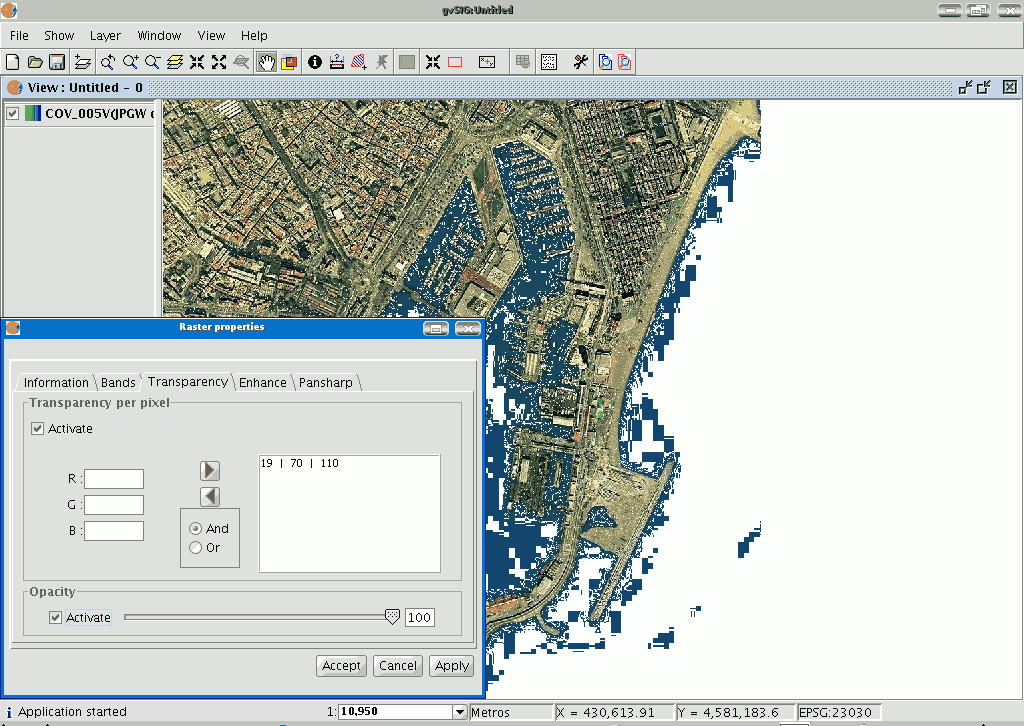
Adding the values with an AND means that all the pixels that have the red, green and blue values we have input will become transparent. Adding the values with an OR means that all the pixels that have the red or green or blue values we have input will become transparent. If you select an entry from the list and click on the left-facing arrow, the values will appear in the text boxes and can be modified.
You can input multiple values in the list. This means that when you accept the operation all the pixels whose colour coincides with the values input in the list will be transformed.
Seleccionar capas ráster
This tool allows you to select raster layers from the view and for them to be selected in the ToC. This is useful if you are using an orthophoto mosaic and you need to find out exactly which orthophoto you are working with. You can access this tool from the tool bar by clicking on the following button

or by going to the “View” menu then to “Selection”.
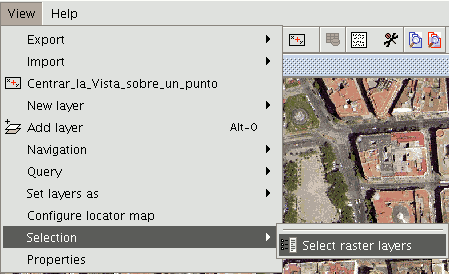
We are now going to show an example of the use of the tool. Remember that there are a large number of orthophotos in the ToC with similar names which as a whole make up the province of Valencia in the “View”.
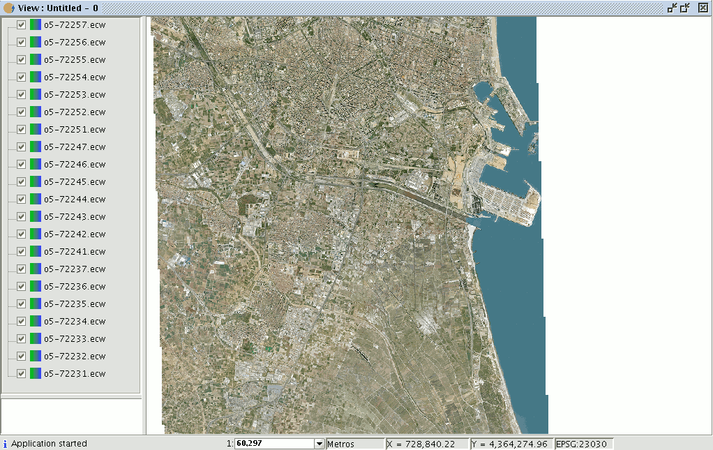
Go to the view. Make sure the selection tool for the raster layer is active and click on the orthophoto you wish to work with.
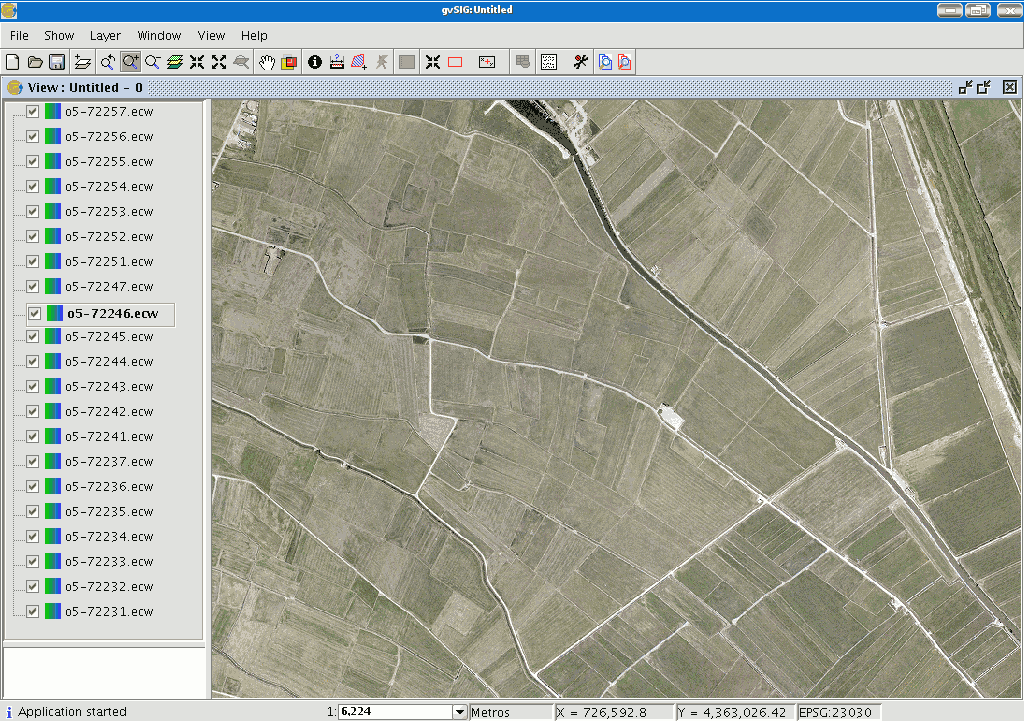
You will see that the chosen orthophoto has automatically been selected in the ToC.
